9.5: Significance Test for a Proportion
- Page ID
- 5787
\( \newcommand{\vecs}[1]{\overset { \scriptstyle \rightharpoonup} {\mathbf{#1}} } \)
\( \newcommand{\vecd}[1]{\overset{-\!-\!\rightharpoonup}{\vphantom{a}\smash {#1}}} \)
\( \newcommand{\dsum}{\displaystyle\sum\limits} \)
\( \newcommand{\dint}{\displaystyle\int\limits} \)
\( \newcommand{\dlim}{\displaystyle\lim\limits} \)
\( \newcommand{\id}{\mathrm{id}}\) \( \newcommand{\Span}{\mathrm{span}}\)
( \newcommand{\kernel}{\mathrm{null}\,}\) \( \newcommand{\range}{\mathrm{range}\,}\)
\( \newcommand{\RealPart}{\mathrm{Re}}\) \( \newcommand{\ImaginaryPart}{\mathrm{Im}}\)
\( \newcommand{\Argument}{\mathrm{Arg}}\) \( \newcommand{\norm}[1]{\| #1 \|}\)
\( \newcommand{\inner}[2]{\langle #1, #2 \rangle}\)
\( \newcommand{\Span}{\mathrm{span}}\)
\( \newcommand{\id}{\mathrm{id}}\)
\( \newcommand{\Span}{\mathrm{span}}\)
\( \newcommand{\kernel}{\mathrm{null}\,}\)
\( \newcommand{\range}{\mathrm{range}\,}\)
\( \newcommand{\RealPart}{\mathrm{Re}}\)
\( \newcommand{\ImaginaryPart}{\mathrm{Im}}\)
\( \newcommand{\Argument}{\mathrm{Arg}}\)
\( \newcommand{\norm}[1]{\| #1 \|}\)
\( \newcommand{\inner}[2]{\langle #1, #2 \rangle}\)
\( \newcommand{\Span}{\mathrm{span}}\) \( \newcommand{\AA}{\unicode[.8,0]{x212B}}\)
\( \newcommand{\vectorA}[1]{\vec{#1}} % arrow\)
\( \newcommand{\vectorAt}[1]{\vec{\text{#1}}} % arrow\)
\( \newcommand{\vectorB}[1]{\overset { \scriptstyle \rightharpoonup} {\mathbf{#1}} } \)
\( \newcommand{\vectorC}[1]{\textbf{#1}} \)
\( \newcommand{\vectorD}[1]{\overrightarrow{#1}} \)
\( \newcommand{\vectorDt}[1]{\overrightarrow{\text{#1}}} \)
\( \newcommand{\vectE}[1]{\overset{-\!-\!\rightharpoonup}{\vphantom{a}\smash{\mathbf {#1}}}} \)
\( \newcommand{\vecs}[1]{\overset { \scriptstyle \rightharpoonup} {\mathbf{#1}} } \)
\(\newcommand{\longvect}{\overrightarrow}\)
\( \newcommand{\vecd}[1]{\overset{-\!-\!\rightharpoonup}{\vphantom{a}\smash {#1}}} \)
\(\newcommand{\avec}{\mathbf a}\) \(\newcommand{\bvec}{\mathbf b}\) \(\newcommand{\cvec}{\mathbf c}\) \(\newcommand{\dvec}{\mathbf d}\) \(\newcommand{\dtil}{\widetilde{\mathbf d}}\) \(\newcommand{\evec}{\mathbf e}\) \(\newcommand{\fvec}{\mathbf f}\) \(\newcommand{\nvec}{\mathbf n}\) \(\newcommand{\pvec}{\mathbf p}\) \(\newcommand{\qvec}{\mathbf q}\) \(\newcommand{\svec}{\mathbf s}\) \(\newcommand{\tvec}{\mathbf t}\) \(\newcommand{\uvec}{\mathbf u}\) \(\newcommand{\vvec}{\mathbf v}\) \(\newcommand{\wvec}{\mathbf w}\) \(\newcommand{\xvec}{\mathbf x}\) \(\newcommand{\yvec}{\mathbf y}\) \(\newcommand{\zvec}{\mathbf z}\) \(\newcommand{\rvec}{\mathbf r}\) \(\newcommand{\mvec}{\mathbf m}\) \(\newcommand{\zerovec}{\mathbf 0}\) \(\newcommand{\onevec}{\mathbf 1}\) \(\newcommand{\real}{\mathbb R}\) \(\newcommand{\twovec}[2]{\left[\begin{array}{r}#1 \\ #2 \end{array}\right]}\) \(\newcommand{\ctwovec}[2]{\left[\begin{array}{c}#1 \\ #2 \end{array}\right]}\) \(\newcommand{\threevec}[3]{\left[\begin{array}{r}#1 \\ #2 \\ #3 \end{array}\right]}\) \(\newcommand{\cthreevec}[3]{\left[\begin{array}{c}#1 \\ #2 \\ #3 \end{array}\right]}\) \(\newcommand{\fourvec}[4]{\left[\begin{array}{r}#1 \\ #2 \\ #3 \\ #4 \end{array}\right]}\) \(\newcommand{\cfourvec}[4]{\left[\begin{array}{c}#1 \\ #2 \\ #3 \\ #4 \end{array}\right]}\) \(\newcommand{\fivevec}[5]{\left[\begin{array}{r}#1 \\ #2 \\ #3 \\ #4 \\ #5 \\ \end{array}\right]}\) \(\newcommand{\cfivevec}[5]{\left[\begin{array}{c}#1 \\ #2 \\ #3 \\ #4 \\ #5 \\ \end{array}\right]}\) \(\newcommand{\mattwo}[4]{\left[\begin{array}{rr}#1 \amp #2 \\ #3 \amp #4 \\ \end{array}\right]}\) \(\newcommand{\laspan}[1]{\text{Span}\{#1\}}\) \(\newcommand{\bcal}{\cal B}\) \(\newcommand{\ccal}{\cal C}\) \(\newcommand{\scal}{\cal S}\) \(\newcommand{\wcal}{\cal W}\) \(\newcommand{\ecal}{\cal E}\) \(\newcommand{\coords}[2]{\left\{#1\right\}_{#2}}\) \(\newcommand{\gray}[1]{\color{gray}{#1}}\) \(\newcommand{\lgray}[1]{\color{lightgray}{#1}}\) \(\newcommand{\rank}{\operatorname{rank}}\) \(\newcommand{\row}{\text{Row}}\) \(\newcommand{\col}{\text{Col}}\) \(\renewcommand{\row}{\text{Row}}\) \(\newcommand{\nul}{\text{Nul}}\) \(\newcommand{\var}{\text{Var}}\) \(\newcommand{\corr}{\text{corr}}\) \(\newcommand{\len}[1]{\left|#1\right|}\) \(\newcommand{\bbar}{\overline{\bvec}}\) \(\newcommand{\bhat}{\widehat{\bvec}}\) \(\newcommand{\bperp}{\bvec^\perp}\) \(\newcommand{\xhat}{\widehat{\xvec}}\) \(\newcommand{\vhat}{\widehat{\vvec}}\) \(\newcommand{\uhat}{\widehat{\uvec}}\) \(\newcommand{\what}{\widehat{\wvec}}\) \(\newcommand{\Sighat}{\widehat{\Sigma}}\) \(\newcommand{\lt}{<}\) \(\newcommand{\gt}{>}\) \(\newcommand{\amp}{&}\) \(\definecolor{fillinmathshade}{gray}{0.9}\)Significance Testing for Proportions
We have studied the test statistic that is used when you are testing hypotheses about the mean of a population and you have a large sample (>30).
Often statisticians are interest in making inferences about a population proportion. For example, when we look at election results we often look at the proportion of people that vote and who this proportion of voters choose. Typically, we call these proportions percentages and we would say something like “Approximately 68 percent of the population voted in this election and 48 percent of these voters voted for Barack Obama.”
So how do we test hypotheses about proportions? We use the same process as we did when testing hypotheses about populations but we must include sample proportions as part of the analysis. This Concept will address how we investigate hypotheses around population proportions and how to construct confidence intervals around our results.
Hypothesis Testing about Population Proportions by Applying the Binomial Distribution Approximation
We could perform tests of population proportions to answer the following questions:
- What percentage of graduating seniors will attend a 4-year college?
- What proportion of voters will vote for John McCain?
- What percentage of people will choose Diet Pepsi over Diet Coke?
To test questions like these, we make hypotheses about population proportions. For example,
H0:35% of graduating seniors will attend a 4-year college.
H0:42% of voters will vote for John McCain.
H0:26% of people will choose Diet Pepsi over Diet Coke.
To test these hypotheses we follow a series of steps:
- Hypothesize a value for the population proportion P like we did above.
- Randomly select a sample.
- Use the sample proportion p̂ to test the stated hypothesis.
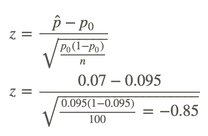
To determine the test statistic we need to know the sampling distribution of the sample proportion. We use the binomial distribution which illustrates situations in which two outcomes are possible (for example, voted for a candidate, didn’t vote for a candidate), remembering that when the sample size is relatively large, we can use the normal distribution to approximate the binomial distribution. The test statistic is

where:
p0 is the hypothesized value of the proportion under the null hypothesis
n is the sample size
Determining Hypotheses and Test Statistics
We want to test a hypothesis that 60 percent of the 400 seniors graduating from a certain California high school will enroll in a two or four-year college upon graduation. What would be our hypotheses and the test statistic?
Since we want to test the proportion of graduating seniors and we think that proportion is around 60 percent, our hypotheses are:
H0:p=.6
Ha:p≠.6
The test statistic would be  . To complete this calculation we would have to have a value for the sample size (n).
Testing a Proportion Hypothesis
Similar to testing hypotheses dealing with population means, we use a similar set of steps when testing proportion hypotheses.
- Determine and state the null and alternative hypotheses.
- Set the criterion for rejecting the null hypothesis.
- Calculate the test statistic.
- Decide whether to reject or fail to reject the null hypothesis.
- Interpret your decision within the context of the problem.
A congressman is trying to decide on whether to vote for a bill that would legalize gay marriage. He will decide to vote for the bill only if 70 percent of his constituents favor the bill. In a survey of 300 randomly selected voters, 224 (74.6%) indicated that they would favor the bill. Should he or should he not vote for the bill?
First, we develop our null and alternative hypotheses.
H0:p=.7
Ha:p>.7
Next, we should set the criterion for rejecting the null hypothesis. Choose α=.05 and since the null hypothesis is considering p>.7, this is a one tailed test. Using a standard z table or the TI 83/84 calculator we find the critical value for a one tailed test at an alpha level of .05 to be 1.645.
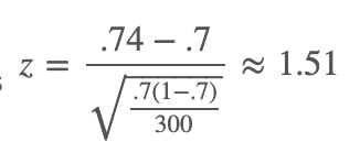
The test statistic is 
Since our critical value is 1.645 and our test statistic is 1. 51, we cannot reject the null hypothesis. This means that we cannot conclude that the population proportion is greater than .70 with 95 percent certainty. Given this information, it is not safe to conclude that at least 70 percent of the voters would favor this bill with any degree of certainty. Even though the proportion of voters supporting the bill is over 70 percent, this could be due to chance and is not statistically significant.
Evaluating the Accuracy of Predictions
Admission staff from a local university is conducting a survey to determine the proportion of incoming freshman that will need financial aid. A survey on housing needs, financial aid and academic interests is collected from 400 of the incoming freshman. Staff hypothesized that 30 percent of freshman will need financial aid and the sample from the survey indicated that 101 (25.3%) would need financial aid. Is this an accurate guess?
First, we develop our null and alternative hypotheses.
H0:p=.3
Ha:p≠.3
Next, we should set the criterion for rejecting the null hypothesis. The .05 alpha level is used and for a two tailed test the critical values of the test statistic are 1.96 and -1.96.
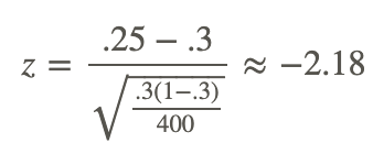
To calculate the test statistic:

Since our critical values are ±1.96 and −2.18<−1.96 we can reject the null hypothesis. This means that we can conclude that the population of freshman needing financial aid is significantly more or less than 30 percent. Since the test statistic is negative, we can conclude with 95% certainty that in the population of incoming freshman, less than 30 percent of the students will need financial aid.
Example
Example 1
The National Institute of Mental Health published an article stating that in any one-year period, approximately 9.5% of American adults suffer from depression or a depressive illness. Suppose that in a survey of 100 people, seven of them suffered from depression or a depressive illness. Conduct a hypothesis test to determine if the true proportion of people is lower than the percent in the general adult American population.
The null and alternative hypotheses are:
H0:p=0.095
H0:p<0.095
The sample proportion is:
p̂ =0.07
The test statistic is:

The p-value is the probability of having a z this extreme or more extreme given the null hypothesis is true. To determine the p-value you can use the TI Calculator and normcdf(-1000000,-.85,0,1) = .198. Since this value is greater than .05 we accept the null hypothesis. Another way to determine the decision is to choose . This is a one sided test and we are going to reject the null hypothesis for small values of the test statistic. (This is based on the direction of the alternative hypothesis). The critical value for this alpha level is -1.96. Any test statistic value less than -1.96 will be in the rejection region and any value greater than -1.96 will be in the acceptance region. Our test statistic value (-.85) is greater than -1.96 and thus is in the acceptance region. Thus, we fail to reject the null hypothesis and believe the true proportion of people with depressive illness is not lower than the general population.
Review
- A college bookstore is trying to decide how many graphing calculators to rent to students taking statistics classes. They believe that a majority of statistics students are interested in renting a graphing calculators. State the null and alternative hypotheses.
- The test statistic helps us determine ___.
- True or false: In statistics, we are able to study and make inferences about proportions, or percentages, of a population.
- A state senator cannot decide how to vote on an environmental protection bill. The senator decides to request her own survey and if the proportion of registered voters supporting the bill exceeds 0.60, she will vote for it. A random sample of 750 voters is selected and 495 are found to support the bill.
- What are the null and alternative hypotheses for this problem?
- What is the observed value of the sample proportion?
- What is the standard error of the proportion?
- What is the test statistic for this scenario?
- What decision would you make about the null hypothesis if you had an alpha level of .01?
- A large city is thinking about a ban on smoking in public places. The city council wants to institute the ban only if more than 75% of the adults living in the city support the ban. To find out if this is so, the city conducts a survey, randomly selecting 200 adults who live in the city and asking them if they would support the ban. Of the 200 adults questioned, 112 said that they support the ban. Is there sufficient statistical evidence to conclude there is strong enough support for the ban among the city’s residents?
- A banker claims that 30% of the loans given by his bank are student loans. A random sample of 64 loans is drawn. It is found that 43 of these are student loans. At the 5% level of significance, test the banker’s assertion.
- A hotel claims that the percentage of vacant rooms each night is 30%. A random survey is taken of 150 rooms found that 31 were empty. At the 2% level of significance test the claim.
- A restaurant owner claims that the percentage of customers who want desert after a meal is less than or equal to 50%. A random sample of 150 customers finds that 81 want desert. At the 1% level of significance test the claim of the restaurant owner.
- A drug company claims that is has developed a drug that will be effective for more than 70% of the patients suffering from high blood pressure. When 60 such patients are given the drug it is effective for 29 of them. What can you conclude?
- About 10% of the population is left-handed. A researcher believes that journalists are more likely to be left-handed than other people in the general population. The researcher surveys 200 journalists and finds that 25 of them are left-handed. Conduct an hypothesis test to determine if the researcher’s claim can be accepted.
- Suppose a drug company wants to claim that the side effects of a medication they are selling will be experienced by fewer than 10% of people taking the medication. In a clinical trial with 300 patients they find that 54 of the patients experienced side effects. Perform an hypothesis test to determine if the company’s claim is accurate.
- Suppose in a survey it is determined that 55% of 70 participants preferred product A over product B. Using this data, test the hypothesis that there is no preference for either of the products.
- A politician is trying to decide whether or not to support a particular bill in Congress. In a random sample of 200 voters in her district, 83 indicate they support the new bill. Should the politician vote in support of the new bill?
- A video rental store claims that the proportion of rentals to college students is at least 60%. A random sample of 164 customers finds that 81 college students rented videos. Test the store’s claim at the 2% level of significance.
- A lumberjack claims that 35% of the trees that are cut down are maple trees. In a random sample of 150 trees that are cut down, it is found that 23 of them are maple trees. At the 10% level test the lumberjack’s claim.
- A carpenter is increasing his price for projects, claiming that the cost of material is going up and accounts for 70% of his budget. In a random sample of 49 of his projects it is found that in 30 of the projects the cost of the material is higher. At the 5% level of significance, test the carpenter’s claim.
Vocabulary
| Term | Definition |
|---|---|
| confidence intervals | A confidence interval is the interval within which you expect to capture a specific value. The confidence interval width is dependent on the confidence level. |
| hypothesis testing | Hypothesis testing involves testing the difference between a hypothesized value of a population parameter and the estimate of that parameter which is calculated from a sample. |
| hypothesized population proportion | The hypothesized population proportion is given the symbol psubscripto in the z-score calculation. |
| sample proportion | The sample proportion is the proportion of individuals in a sample sharing a certain trait, denoted phat.. |
| test statistic | A test statistic is a single measure of some attribute of a sample (i.e. a statistic) used in statistical hypothesis testing. The z‐score is one kind of test statistic that is used to determine the probability of obtaining a given value. |
Additional Resources
Video: Sampling Distribution of Sample Proportion
Practice: Significance Test for a Proportion

