
9.7: Dependent and Independent Samples
- Page ID
- 5789
\( \newcommand{\vecs}[1]{\overset { \scriptstyle \rightharpoonup} {\mathbf{#1}} } \)
\( \newcommand{\vecd}[1]{\overset{-\!-\!\rightharpoonup}{\vphantom{a}\smash {#1}}} \)
\( \newcommand{\dsum}{\displaystyle\sum\limits} \)
\( \newcommand{\dint}{\displaystyle\int\limits} \)
\( \newcommand{\dlim}{\displaystyle\lim\limits} \)
\( \newcommand{\id}{\mathrm{id}}\) \( \newcommand{\Span}{\mathrm{span}}\)
( \newcommand{\kernel}{\mathrm{null}\,}\) \( \newcommand{\range}{\mathrm{range}\,}\)
\( \newcommand{\RealPart}{\mathrm{Re}}\) \( \newcommand{\ImaginaryPart}{\mathrm{Im}}\)
\( \newcommand{\Argument}{\mathrm{Arg}}\) \( \newcommand{\norm}[1]{\| #1 \|}\)
\( \newcommand{\inner}[2]{\langle #1, #2 \rangle}\)
\( \newcommand{\Span}{\mathrm{span}}\)
\( \newcommand{\id}{\mathrm{id}}\)
\( \newcommand{\Span}{\mathrm{span}}\)
\( \newcommand{\kernel}{\mathrm{null}\,}\)
\( \newcommand{\range}{\mathrm{range}\,}\)
\( \newcommand{\RealPart}{\mathrm{Re}}\)
\( \newcommand{\ImaginaryPart}{\mathrm{Im}}\)
\( \newcommand{\Argument}{\mathrm{Arg}}\)
\( \newcommand{\norm}[1]{\| #1 \|}\)
\( \newcommand{\inner}[2]{\langle #1, #2 \rangle}\)
\( \newcommand{\Span}{\mathrm{span}}\) \( \newcommand{\AA}{\unicode[.8,0]{x212B}}\)
\( \newcommand{\vectorA}[1]{\vec{#1}} % arrow\)
\( \newcommand{\vectorAt}[1]{\vec{\text{#1}}} % arrow\)
\( \newcommand{\vectorB}[1]{\overset { \scriptstyle \rightharpoonup} {\mathbf{#1}} } \)
\( \newcommand{\vectorC}[1]{\textbf{#1}} \)
\( \newcommand{\vectorD}[1]{\overrightarrow{#1}} \)
\( \newcommand{\vectorDt}[1]{\overrightarrow{\text{#1}}} \)
\( \newcommand{\vectE}[1]{\overset{-\!-\!\rightharpoonup}{\vphantom{a}\smash{\mathbf {#1}}}} \)
\( \newcommand{\vecs}[1]{\overset { \scriptstyle \rightharpoonup} {\mathbf{#1}} } \)
\(\newcommand{\longvect}{\overrightarrow}\)
\( \newcommand{\vecd}[1]{\overset{-\!-\!\rightharpoonup}{\vphantom{a}\smash {#1}}} \)
\(\newcommand{\avec}{\mathbf a}\) \(\newcommand{\bvec}{\mathbf b}\) \(\newcommand{\cvec}{\mathbf c}\) \(\newcommand{\dvec}{\mathbf d}\) \(\newcommand{\dtil}{\widetilde{\mathbf d}}\) \(\newcommand{\evec}{\mathbf e}\) \(\newcommand{\fvec}{\mathbf f}\) \(\newcommand{\nvec}{\mathbf n}\) \(\newcommand{\pvec}{\mathbf p}\) \(\newcommand{\qvec}{\mathbf q}\) \(\newcommand{\svec}{\mathbf s}\) \(\newcommand{\tvec}{\mathbf t}\) \(\newcommand{\uvec}{\mathbf u}\) \(\newcommand{\vvec}{\mathbf v}\) \(\newcommand{\wvec}{\mathbf w}\) \(\newcommand{\xvec}{\mathbf x}\) \(\newcommand{\yvec}{\mathbf y}\) \(\newcommand{\zvec}{\mathbf z}\) \(\newcommand{\rvec}{\mathbf r}\) \(\newcommand{\mvec}{\mathbf m}\) \(\newcommand{\zerovec}{\mathbf 0}\) \(\newcommand{\onevec}{\mathbf 1}\) \(\newcommand{\real}{\mathbb R}\) \(\newcommand{\twovec}[2]{\left[\begin{array}{r}#1 \\ #2 \end{array}\right]}\) \(\newcommand{\ctwovec}[2]{\left[\begin{array}{c}#1 \\ #2 \end{array}\right]}\) \(\newcommand{\threevec}[3]{\left[\begin{array}{r}#1 \\ #2 \\ #3 \end{array}\right]}\) \(\newcommand{\cthreevec}[3]{\left[\begin{array}{c}#1 \\ #2 \\ #3 \end{array}\right]}\) \(\newcommand{\fourvec}[4]{\left[\begin{array}{r}#1 \\ #2 \\ #3 \\ #4 \end{array}\right]}\) \(\newcommand{\cfourvec}[4]{\left[\begin{array}{c}#1 \\ #2 \\ #3 \\ #4 \end{array}\right]}\) \(\newcommand{\fivevec}[5]{\left[\begin{array}{r}#1 \\ #2 \\ #3 \\ #4 \\ #5 \\ \end{array}\right]}\) \(\newcommand{\cfivevec}[5]{\left[\begin{array}{c}#1 \\ #2 \\ #3 \\ #4 \\ #5 \\ \end{array}\right]}\) \(\newcommand{\mattwo}[4]{\left[\begin{array}{rr}#1 \amp #2 \\ #3 \amp #4 \\ \end{array}\right]}\) \(\newcommand{\laspan}[1]{\text{Span}\{#1\}}\) \(\newcommand{\bcal}{\cal B}\) \(\newcommand{\ccal}{\cal C}\) \(\newcommand{\scal}{\cal S}\) \(\newcommand{\wcal}{\cal W}\) \(\newcommand{\ecal}{\cal E}\) \(\newcommand{\coords}[2]{\left\{#1\right\}_{#2}}\) \(\newcommand{\gray}[1]{\color{gray}{#1}}\) \(\newcommand{\lgray}[1]{\color{lightgray}{#1}}\) \(\newcommand{\rank}{\operatorname{rank}}\) \(\newcommand{\row}{\text{Row}}\) \(\newcommand{\col}{\text{Col}}\) \(\renewcommand{\row}{\text{Row}}\) \(\newcommand{\nul}{\text{Nul}}\) \(\newcommand{\var}{\text{Var}}\) \(\newcommand{\corr}{\text{corr}}\) \(\newcommand{\len}[1]{\left|#1\right|}\) \(\newcommand{\bbar}{\overline{\bvec}}\) \(\newcommand{\bhat}{\widehat{\bvec}}\) \(\newcommand{\bperp}{\bvec^\perp}\) \(\newcommand{\xhat}{\widehat{\xvec}}\) \(\newcommand{\vhat}{\widehat{\vvec}}\) \(\newcommand{\uhat}{\widehat{\uvec}}\) \(\newcommand{\what}{\widehat{\wvec}}\) \(\newcommand{\Sighat}{\widehat{\Sigma}}\) \(\newcommand{\lt}{<}\) \(\newcommand{\gt}{>}\) \(\newcommand{\amp}{&}\) \(\definecolor{fillinmathshade}{gray}{0.9}\)Testing a Hypothesis for Dependent and Independent Samples
Hypothesis Testing for Dependent and Independent Samples
We have learned about hypothesis testing for proportion and means with both large and small samples. However, in the examples in those lessons only one sample was involved. In this lesson we will apply the principals of hypothesis testing to situations involving two samples. There are many situations in everyday life where we would perform statistical analysis involving two samples. For example, suppose that we wanted to test a hypothesis about the effect of two medications on curing an illness. Or we may want to test the difference between the means of males and females on the SAT. In both of these cases, we would analyze both samples and the hypothesis would address the difference between two sample means.
In this Concept, we will identify situations with different types of samples, learn to calculate the test statistic, calculate the estimate for population variance for both samples and calculate the test statistic to test hypotheses about the difference of proportions or means between samples.
Dependent and Independent Samples
When we are working with one sample, we know that we need to select a random sample from the population, measure that sample statistic and then make hypothesis about the population based on that sample. When we work with two independent samples we assume that if the samples are selected at random (or, in the case of medical research, the subjects are randomly assigned to a group), the two samples will vary only by chance and the difference will not be statistically significant. In short, when we have independent samples we assume that the scores of one sample do not affect the other.
Independent samples can occur in two scenarios.
Testing the difference of the means between two fixed populations we test the differences between samples from each population. When both samples are randomly selected, we can make inferences about the populations.
When working with subjects (people, pets, etc.), if we select a random sample and then randomly assign half of the subjects to one group and half to another we can make inferences about the populations.
Dependent samples are a bit different. Two samples of data are dependent when each score in one sample is paired with a specific score in the other sample. In short, these types of samples are related to each other. Dependent samples can occur in two scenarios. In one, a group may be measured twice such as in a pretest-posttest situation (scores on a test before and after the lesson). The other scenario is one in which an observation in one sample is matched with an observation in the second sample.
To distinguish between tests of hypotheses for independent and dependent samples, we use a different symbol for hypotheses with dependent samples. For dependent sample hypotheses, we use the delta symbol δ to symbolize the difference between the two samples. Therefore, in our null hypothesis we state that the difference of scores across the two measurements is equal to 0;δ=0 or:
H0:δ=μ1−μ2
Calculating the Pooled Estimate of Population Variance
When testing a hypothesis about two independent samples, we follow a similar process as when testing one random sample. However, when computing the test statistic, we need to calculate the estimated standard error of the difference between sample means,
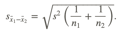
Where n1 and n2 are the sizes of the two samples s2 is the pooled sample variance, which is computed as 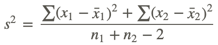 . Often, the top part of this formula is simplified by substituting the symbol SS for the sum of the squared deviations. Therefore, the formula often is expressed by
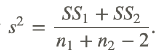
Calculating s2 Suppose we have two independent samples of student reading scores.
The data are as follows:
| Sample 1 | Sample 2 |
|---|---|
| 7 | 12 |
| 8 | 14 |
| 10 | 18 |
| 4 | 13 |
| 6 | 11 |
| 10 |
From this sample, we can calculate a number of descriptive statistics that will help us solve for the pooled estimate of variance:
| Descriptive Statistic | Sample 1 | Sample 2 |
|---|---|---|
| Number n | 5 | 6 |
| Sum of Observations ∑x | 35 | 78 |
| Mean of Observations x̄ | 7 | 13 |
| Sum of Squared Deviations ∑(xi−x̄)2 {i:1,n} | 20 | 40 |
Using the formula for the pooled estimate of variance, we find that
s2=6.67
We will use this information to calculate the test statistic needed to evaluate the hypotheses.
Testing Hypotheses with Independent Samples
When testing hypotheses with two independent samples, we follow similar steps as when testing one random sample:
- State the null and alternative hypotheses.
- Choose α
- Set the criterion (critical values) for rejecting the null hypothesis.
- Compute the test statistic.
- Make a decision: reject or fail to reject the null hypothesis.
- Interpret the decision within the context of the problem.
When stating the null hypothesis, we assume there is no difference between the means of the two independent samples. Therefore, our null hypothesis in this case would be:
H0:μ1=μ2 or H0:μ1−μ2=0
Similar to the one-sample test, the critical values that we set to evaluate these hypotheses depend on our alpha level and our decision regarding the null hypothesis is carried out in the same manner. However, since we have two samples, we calculate the test statistic a bit differently and use the formula:
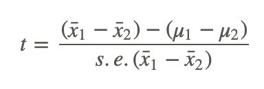
where:
x̄1−x̄2 is the difference between the sample means
μ1−μ2 is the difference between the hypothesized population means
s.e.(x̄1−x̄2) is the standard error of the difference between sample means
Evaluating the Difference Between Two Samples
The head of the English department is interested in the difference in writing scores between remedial freshman English students who are taught by different teachers. The incoming freshmen needing remedial services are randomly assigned to one of two English teachers and are given a standardized writing test after the first semester. We take a sample of eight students from one class and nine from the other. Is there a difference in achievement on the writing test between the two classes? Use a 0.05 significance level.
First, we would generate our hypotheses based on the two samples.
H0:μ1=μ2
Ha:μ1≠μ2
This is a two tailed test. For this example, we have two independent samples from the population and have a total of 17 students that we are examining. Since our sample size is so low, we use the t−distribution. In this example, we have 15 degrees of freedom (number in the samples minus 2) and with a .05 significance level and the t distribution, we find that our critical values are 2.131 standard scores above and below the mean.
To calculate the test statistic, we first need to find the pooled estimate of variance from our sample. The data from the two groups are as follows:
| Sample 1 | Sample 2 |
|---|---|
| 35 | 52 |
| 51 | 87 |
| 66 | 76 |
| 42 | 62 |
| 37 | 81 |
| 46 | 71 |
| 60 | 55 |
| 55 | 67 |
| 53 |
From this sample, we can calculate several descriptive statistics that will help us solve for the pooled estimate of variance:
| Descriptive Statistic | Sample 1 | Sample 2 |
|---|---|---|
| Number n | 9 | 8 |
| Sum of Observations ∑x | 445 | 551 |
| Mean of Observations x̄ | 49.44 | 68.875 |
| Sum of Squared Deviations ∑(xi−x̄)2 from {i:1,n} | 862.22 | 1058.88 |
Therefore:
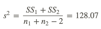
and the standard error of the difference of the sample means is:
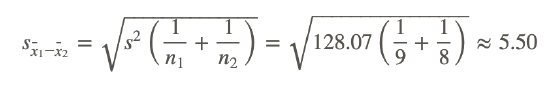
Using this information, we can finally solve for the test statistic:
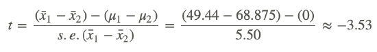
Since -3.53 is less than the critical value of 2.13, we decide to reject the null hypothesis and conclude there is a significant difference in the achievement of the students assigned to different teachers.
Testing Hypotheses about the Difference in Proportions between Two Independent Samples
Suppose we want to test if there is a difference between proportions of two independent samples. As discussed in the previous lesson, proportions are used extensively in polling and surveys, especially by people trying to predict election results. It is possible to test a hypothesis about the proportions of two independent samples by using a similar method as described above. We might perform these hypotheses tests in the following scenarios:
- When examining the proportion of children living in poverty in two different towns.
- When investigating the proportions of freshman and sophomore students who report test anxiety.
- When testing if the proportion of high school boys and girls who smoke cigarettes is equal.
In testing hypotheses about the difference in proportions of two independent samples, we state the hypotheses and set the criterion for rejecting the null hypothesis in similar ways as the other hypotheses tests. In these types of tests we set the proportions of the samples equal to each other in the null hypothesis H0:p1=p2 and use the appropriate standard table to determine the critical values (remember, for small samples we generally use the t distribution and for samples over 30 we generally use the z−distribution).
When solving for the test statistic in large samples, we use the formula:
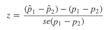
where:
p̂ 1,p̂ 2 are the observed sample proportions
p1,p2 are the population proportions under the null hypothesis
se(p1−p2) is the standard error of the difference between independent proportions
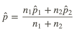
Similar to the standard error of the difference between independent samples, we need to do a bit of work to calculate the standard error of the difference between independent proportions. To find the standard error under the null hypothesis we assume that p1=p2=p and we use all the data to estimate p.
Now the standard error of the difference is 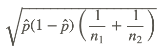
The test statistic is now 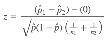
Determining Statistical Difference
Suppose that we are interested in finding out which particular city is more is more satisfied with the services provided by the city government. We take a survey and find the following results:
| Number Satisfied | City 1 | City 2 |
|---|---|---|
| Yes | 122 | 84 |
| No | 78 | 66 |
| Sample Size | n1=200 | n2=150 |
| Proportion who said Yes | 0.61 | 0.56 |
Is there a statistical difference in the proportions of citizens that are satisfied with the services provided by the city government? Use a 0.05 level of significance.
First, we establish the null and alternative hypotheses:
H0:p1=p2
Ha:p1≠p2
Since we have a large sample size we will use the z−distribution. At a .05 level of significance, our critical values are ±1.96. To solve for the test statistic, we must first solve for the standard error of the difference between proportions.
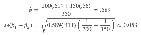
Therefore, the test statistic is:
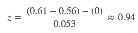
Since 0.94 does not exceed the critical value 1.96, the null hypothesis is not rejected. Therefore, we can conclude that the difference in the probabilities could have occurred by chance and that there is no difference in the level of satisfaction between citizens of the two cities.
Testing Hypotheses with Dependent Samples
When testing a hypothesis about two dependent samples, we follow the same process as when testing one random sample or two independent samples:
- State the null and alternative hypotheses.
- Choose the level of significance
- Set the criterion (critical values) for rejecting the null hypothesis.
- Compute the test statistic.
- Make a decision, reject or fail to reject the null hypothesis
- Interpret our results.
As mentioned in the section above, our hypothesis for two dependent samples states that there is no difference between the scores across the two samples H0:δ=μ1−μ2=0. We set the criterion for evaluating the hypothesis in the same way that we do with our other examples – by first establishing an alpha level and then finding the critical values by using the t−distribution table. Calculating the test statistic for dependent samples is a bit different since we are dealing with two sets of data. The test statistic that we first need calculate is  , which is the difference in the means of the two samples. Therefore, =x̄1−x̄2. We also need to know the standard error of the difference between the two samples. Since our population variance is unknown, we estimate it by first using the formula for the standard deviations of the samples:
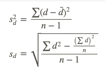
where:
s2d is the sample variance
d is the difference between corresponding pairs within the sample
is the difference between the means of the two samples
n is the number in the sample
sd is the standard deviation
With the standard deviation, we can calculate the standard error using the following formula:
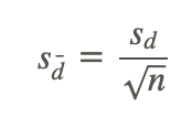
After we calculate the standard error, we can use the general formula for the test statistic:
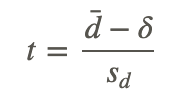
Evaluating the Relationship Between Two Samples
The math teacher wants to determine the effectiveness of her statistics lesson and gives a pre-test and a post-test to 9 students in her class. Our hypothesis is that there is no difference between the means of the two samples and our alternative hypothesis is that the two means of the samples are not equal. In other words, we are testing whether or not these two samples are related or:
H0:δ=μ1−μ2=0
Ha:δ=μ1−μ2≠0
The results for the pre-and post-tests are below:
| Subject | Pre-test Score | Post-test Score | d difference | d2 |
|---|---|---|---|---|
| 1 | 78 | 80 | 2 | 4 |
| 2 | 67 | 69 | 2 | 4 |
| 3 | 56 | 70 | 14 | 196 |
| 4 | 78 | 79 | 1 | 1 |
| 5 | 96 | 96 | 0 | 0 |
| 6 | 82 | 84 | 2 | 4 |
| 7 | 84 | 88 | 4 | 16 |
| 8 | 90 | 92 | 2 | 4 |
| 9 | 87 | 92 | 5 | 25 |
| Sum | 718 | 750 | 32 | 254 |
| Mean | 79.7 | 83.3 | 3.6 |
Using the information from the table above, first solve for the standard deviation of the two samples, then the standard error of the two samples and finally the test statistic.
Standard Deviation:
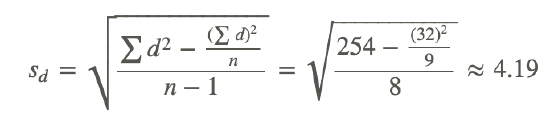
Standard Error of the Difference:
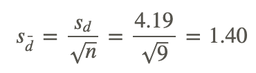
Test Statistic (t−Test)
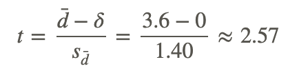
With 8 degrees of freedom (number of observations - 1) and a significance level of .05, we find our critical values to be ±2.306. Since our test statistic exceeds this critical value, we can reject the null hypothesis that the two samples are equal and conclude that the lesson had an effect on student achievement.
Example
Example 1
You have obtained the number of years of education from one random sample of 38 police officers from City A and the number of years of education from a second random sample of 30 police officers from City B. The average years of education for the sample from City A is 15 years with a standard deviation of 2 years. The average years of education for the sample from City B is 14 years with a standard deviation of 2.5 years. Is there a statistically significant difference between the education levels of police officers in City A and City B?
First, find the test statistic:
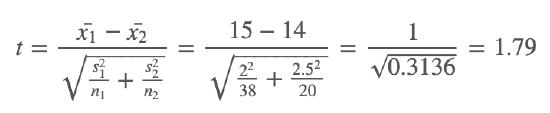
This is a t – statistic with 66 degrees of freedom. This is a two-sided test, with the p-value = 0.07. Since this is greater than .05 we fail to reject the null hypothesis. This means that we believe there is no statistically significant difference between the education levels of police officers in the two different cities.
Review
- In hypothesis testing, we have scenarios that have both dependent and independent samples. Give an example of an experiment with (1) dependent samples and (2) independent samples.
- True or False: When we test the difference between the means of males and females on the SAT, we are using independent samples.
- A study is conducted on the effectiveness of a drug on the hyperactivity of laboratory rats. Two random samples of rats are used for the study and one group is given Drug A and the other group is given Drug B and the number of times that they push a lever is recorded. The following results for this test were calculated:
| Drug A | Drug B | |
|---|---|---|
| X | 75.6 | 72.8 |
| n | 18 | 24 |
| s2 | 12.25 | 10.24 |
| s | 3.5 | 3.2 |
(a) Does this scenario involve dependent or independent samples? Explain.
(b) What would the hypotheses be for this scenario?
(c) Compute the pooled estimate for population variance.
(d) Calculate the estimated standard error for this scenario.
(e) What is the test statistic and at an alpha level of .05 what conclusions would you make about the null hypothesis?
- A survey is conducted on attitudes towards drinking. A random sample of eight married couples is selected, and the husbands and wives respond to an attitude-toward-drinking scale. The scores are as follows:
| Husbands | Wives |
|---|---|
| 16 | 15 |
| 20 | 18 |
| 10 | 13 |
| 15 | 10 |
| 8 | 12 |
| 19 | 16 |
| 14 | 11 |
| 15 | 12 |
(a) What would be the hypotheses for this scenario?
(b) Calculate the estimated standard deviation for this scenario.
(c) Compute the standard error of the difference for these samples.
(d) What is the test statistic and at an alpha level of .05 what conclusions would you make about the null hypothesis?
- In a random sample of 160 couples, the difference between the husband and wife’s ages had a mean of 2.24 years and a standard deviation of 4.1 years. Test the hypothesis that men are significantly older than their wives, on average.
- For each of the following determine if a paired t-test or a two-sample t-test is appropriate:
- The weights of marathon runners were taken before and after a run to test if runners lose dangerous levels of fluid.
- Do levels of knowledge about current events differ between freshmen and juniors in college?
- Calculate the value of the test statistic t in each of the following situations. In each case the null hypothesis is the same:
- x̄1=35,s1=10,n1=100,x̄2=33,s2=9,n2=81
- The difference between the sample means is 52, the standard error of the difference between the sample means is 24.
- Consider the following data. Assume the data comes from appropriate random samples:
Data set A: 188.5 183 194.5 185 214. 205.5 187 183.5
Data set B: 188 185.5 207 188.5 196.5 204.5 180 187
Test the hypothesis that the means of the two populations are equal versus that they are not equal. - A sociologist is interested in determining of the life expectancy of people in Asia is greater than the life expectancy of people in Africa. In a sample of 42 Asians the mean life expectancy was 65.2 years with a standard deviation of 9.3 years. In the sample of 53 Africans the mean life expectancy was 55.3 years with a standard deviation of 8.1 years. Test the hypothesis at the .01 level of significance.
- In each of the following determine whether the alternative hypothesis was the difference in means is greater than zero, or the difference in means is less than zero, or the difference in means is not equal to zero.
- H0:μ1−μ2=0,t=2.33,df=8,p−value=0.048
- H0:μ1−μ2=0,t=−2.33,df=8,p−value=0.024
- H0:μ1−μ2=0,t=−2.33,df=8,p−value=0.976
- A manufacturer is testing two different designs for an air tank. This involves observing how much pressure the tank can withstand before it bursts. For design A, four tanks are sampled and the average pressure to failure was 1500 psi with a standard deviation 250 psi. For design B, six tanks were sampled and had an average pressure to failure of 1610 psi with a standard deviation of 240 psi. Test for a difference in mean pressure to failure for the two designs at the 10% level of significance. Assume the two populations are normally distributed and have the same variance.
- Researchers were studying whether the administration of a growth hormone affects weight gain in pregnant rats. For 6 rats receivng the growth hormone the mean weight gain was 60.8 with a standard deviation of 16.4. For the 6 control rats the weight gain was 41.8 with a standard deviation of 7.6. Is the weight gain for rats receiving the hormone significantly higher than the weight gain in the control group? (source: V.T. Sara, Science 186)
- Do two types of music, type-I and type-II, have different effects upon the ability of college students to perform a series of mental tasks requiring concentration? Thirty college students were randomly divided into two groups of 15 students each. They were asked to perform a series of mental tasks under conditions that are identical in every respect except one: namely, that group A has music of type-I playing in the background, while group B has music of type-II. Following are the results showing how many of the 40 components the students were able to complete.
| Group A: music of type-I | Group B: music of type-II | ||
|---|---|---|---|
| 26 21 22 | 18 23 21 | ||
| 26 19 22 | 20 20 29 | ||
| 26 25 24 | 20 16 20 | ||
| 21 23 23 | 26 21 25 | ||
| 18 29 22 | 17 18 19 |
Complete the hypothesis test to determine if the two types of music have different effects upon the ability of college students to perform a series of mental tasks requiring concentration. (source: Vassar College)
- The campus bookstore asked a random sample of sophomores and juniors how much they spent on textbooks. The bookstore believes the two groups spend the same amount on textbooks. Fifty sophomores had a mean expenditure of $40 with a sample variance of $500 and the 70 juniors sampled had a mean expenditure of $45 with a sample variance of $800. Based on this information is the bookstore’s belief accurate?
- In 1988 Wood, et al, did a study. Eighty-nine sedentary men were given one of two treatments. Forty-two of the men were placed on a diet while forty-seven of them were put on an exercise program. The group on the diet lost an average of 7.2 kg, with a standard deviation of 3.7 kg. The men who exercised lost an average of 4 kg, with a standard deviation of 3.9 kg. Test the hypothesis that the mean weight loss would be different under the two different programs.
- Do the minutes spent exercising in a week differ between men and women in college? To answer this question a random sample of students was taken and the time each spent exercising for a week was recorded. Following is the data that was collected:
Women: 65 243 0 365 455 210 100 72 24 60 64 370 190 3 100 280
Men: 190 310 70 490 0 95 310 176 203 701 300 250
Conduct a test to determine if the mean amount of exercise differs for men and women.
Vocabulary
| Term | Definition |
|---|---|
| dependent samples | Dependent samples occur when you have two samples that do affect one another. |
| independent samples | Independent samples occur when you have two samples that do not affect one another. |
| likelihood | The likelihood is the test statistic (t) associated with two dependent samples. |
| proportions associated with two independent samples | The z-score is the test statistic associated with two independent samples used when testing the proportion associated with two independent samples. |
Additional Resources
Video: t-Test Two Sample for Means Hypothesis Test
Practice: Dependent and Independent Samples