9.10: Tests for Single Variance
- Page ID
- 5792
\( \newcommand{\vecs}[1]{\overset { \scriptstyle \rightharpoonup} {\mathbf{#1}} } \)
\( \newcommand{\vecd}[1]{\overset{-\!-\!\rightharpoonup}{\vphantom{a}\smash {#1}}} \)
\( \newcommand{\dsum}{\displaystyle\sum\limits} \)
\( \newcommand{\dint}{\displaystyle\int\limits} \)
\( \newcommand{\dlim}{\displaystyle\lim\limits} \)
\( \newcommand{\id}{\mathrm{id}}\) \( \newcommand{\Span}{\mathrm{span}}\)
( \newcommand{\kernel}{\mathrm{null}\,}\) \( \newcommand{\range}{\mathrm{range}\,}\)
\( \newcommand{\RealPart}{\mathrm{Re}}\) \( \newcommand{\ImaginaryPart}{\mathrm{Im}}\)
\( \newcommand{\Argument}{\mathrm{Arg}}\) \( \newcommand{\norm}[1]{\| #1 \|}\)
\( \newcommand{\inner}[2]{\langle #1, #2 \rangle}\)
\( \newcommand{\Span}{\mathrm{span}}\)
\( \newcommand{\id}{\mathrm{id}}\)
\( \newcommand{\Span}{\mathrm{span}}\)
\( \newcommand{\kernel}{\mathrm{null}\,}\)
\( \newcommand{\range}{\mathrm{range}\,}\)
\( \newcommand{\RealPart}{\mathrm{Re}}\)
\( \newcommand{\ImaginaryPart}{\mathrm{Im}}\)
\( \newcommand{\Argument}{\mathrm{Arg}}\)
\( \newcommand{\norm}[1]{\| #1 \|}\)
\( \newcommand{\inner}[2]{\langle #1, #2 \rangle}\)
\( \newcommand{\Span}{\mathrm{span}}\) \( \newcommand{\AA}{\unicode[.8,0]{x212B}}\)
\( \newcommand{\vectorA}[1]{\vec{#1}} % arrow\)
\( \newcommand{\vectorAt}[1]{\vec{\text{#1}}} % arrow\)
\( \newcommand{\vectorB}[1]{\overset { \scriptstyle \rightharpoonup} {\mathbf{#1}} } \)
\( \newcommand{\vectorC}[1]{\textbf{#1}} \)
\( \newcommand{\vectorD}[1]{\overrightarrow{#1}} \)
\( \newcommand{\vectorDt}[1]{\overrightarrow{\text{#1}}} \)
\( \newcommand{\vectE}[1]{\overset{-\!-\!\rightharpoonup}{\vphantom{a}\smash{\mathbf {#1}}}} \)
\( \newcommand{\vecs}[1]{\overset { \scriptstyle \rightharpoonup} {\mathbf{#1}} } \)
\(\newcommand{\longvect}{\overrightarrow}\)
\( \newcommand{\vecd}[1]{\overset{-\!-\!\rightharpoonup}{\vphantom{a}\smash {#1}}} \)
\(\newcommand{\avec}{\mathbf a}\) \(\newcommand{\bvec}{\mathbf b}\) \(\newcommand{\cvec}{\mathbf c}\) \(\newcommand{\dvec}{\mathbf d}\) \(\newcommand{\dtil}{\widetilde{\mathbf d}}\) \(\newcommand{\evec}{\mathbf e}\) \(\newcommand{\fvec}{\mathbf f}\) \(\newcommand{\nvec}{\mathbf n}\) \(\newcommand{\pvec}{\mathbf p}\) \(\newcommand{\qvec}{\mathbf q}\) \(\newcommand{\svec}{\mathbf s}\) \(\newcommand{\tvec}{\mathbf t}\) \(\newcommand{\uvec}{\mathbf u}\) \(\newcommand{\vvec}{\mathbf v}\) \(\newcommand{\wvec}{\mathbf w}\) \(\newcommand{\xvec}{\mathbf x}\) \(\newcommand{\yvec}{\mathbf y}\) \(\newcommand{\zvec}{\mathbf z}\) \(\newcommand{\rvec}{\mathbf r}\) \(\newcommand{\mvec}{\mathbf m}\) \(\newcommand{\zerovec}{\mathbf 0}\) \(\newcommand{\onevec}{\mathbf 1}\) \(\newcommand{\real}{\mathbb R}\) \(\newcommand{\twovec}[2]{\left[\begin{array}{r}#1 \\ #2 \end{array}\right]}\) \(\newcommand{\ctwovec}[2]{\left[\begin{array}{c}#1 \\ #2 \end{array}\right]}\) \(\newcommand{\threevec}[3]{\left[\begin{array}{r}#1 \\ #2 \\ #3 \end{array}\right]}\) \(\newcommand{\cthreevec}[3]{\left[\begin{array}{c}#1 \\ #2 \\ #3 \end{array}\right]}\) \(\newcommand{\fourvec}[4]{\left[\begin{array}{r}#1 \\ #2 \\ #3 \\ #4 \end{array}\right]}\) \(\newcommand{\cfourvec}[4]{\left[\begin{array}{c}#1 \\ #2 \\ #3 \\ #4 \end{array}\right]}\) \(\newcommand{\fivevec}[5]{\left[\begin{array}{r}#1 \\ #2 \\ #3 \\ #4 \\ #5 \\ \end{array}\right]}\) \(\newcommand{\cfivevec}[5]{\left[\begin{array}{c}#1 \\ #2 \\ #3 \\ #4 \\ #5 \\ \end{array}\right]}\) \(\newcommand{\mattwo}[4]{\left[\begin{array}{rr}#1 \amp #2 \\ #3 \amp #4 \\ \end{array}\right]}\) \(\newcommand{\laspan}[1]{\text{Span}\{#1\}}\) \(\newcommand{\bcal}{\cal B}\) \(\newcommand{\ccal}{\cal C}\) \(\newcommand{\scal}{\cal S}\) \(\newcommand{\wcal}{\cal W}\) \(\newcommand{\ecal}{\cal E}\) \(\newcommand{\coords}[2]{\left\{#1\right\}_{#2}}\) \(\newcommand{\gray}[1]{\color{gray}{#1}}\) \(\newcommand{\lgray}[1]{\color{lightgray}{#1}}\) \(\newcommand{\rank}{\operatorname{rank}}\) \(\newcommand{\row}{\text{Row}}\) \(\newcommand{\col}{\text{Col}}\) \(\renewcommand{\row}{\text{Row}}\) \(\newcommand{\nul}{\text{Nul}}\) \(\newcommand{\var}{\text{Var}}\) \(\newcommand{\corr}{\text{corr}}\) \(\newcommand{\len}[1]{\left|#1\right|}\) \(\newcommand{\bbar}{\overline{\bvec}}\) \(\newcommand{\bhat}{\widehat{\bvec}}\) \(\newcommand{\bperp}{\bvec^\perp}\) \(\newcommand{\xhat}{\widehat{\xvec}}\) \(\newcommand{\vhat}{\widehat{\vvec}}\) \(\newcommand{\uhat}{\widehat{\uvec}}\) \(\newcommand{\what}{\widehat{\wvec}}\) \(\newcommand{\Sighat}{\widehat{\Sigma}}\) \(\newcommand{\lt}{<}\) \(\newcommand{\gt}{>}\) \(\newcommand{\amp}{&}\) \(\definecolor{fillinmathshade}{gray}{0.9}\)Tests of Single Variance
We have learned how the chi-square test can help us assess the relationships between two variables. In addition to assessing these relationships, the chi-square test can also help us test hypotheses surrounding variance, which is the measure of the variation, or scattering, of scores in a distribution. There are several different tests that we can use to assess the variance of a sample. The most common tests used to assess variance are the chi-square test for one variance, the F-test, and the Analysis of Variance (ANOVA). Both the chi-square test and the F-test are extremely sensitive to non-normality (or when the populations do not have a normal distribution), so the ANOVA test is used most often for this analysis. However, in this Concept, we will examine in greater detail the testing of a single variance using the chi-square test.
Testing a Single Variance Hypothesis Using the Chi-Square Test
Suppose that we want to test two samples to determine if they belong to the same population. The test of variance between samples is used quite frequently in the manufacturing of food, parts, and medications, since it is necessary for individual products of each of these types to be very similar in size and chemical make-up. This test is called the test for one variance.
To perform the test for one variance using the chi-square distribution, we need several pieces of information. First, as mentioned, we should check to make sure that the population has a normal distribution. Next, we need to determine the number of observations in the sample. The remaining pieces of information that we need are the standard deviation and the hypothetical population variance. For the purposes of this exercise, we will assume that we will be provided with the standard deviation and the population variance.
Using these key pieces of information, we use the following formula to calculate the chi-square value to test a hypothesis surrounding single variance:
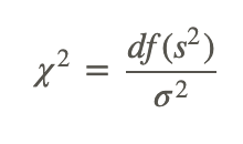
where:
χ2 is the chi-square statistical value.
df=n−1, where n is the size of the sample.
s2 is the sample variance.
σ2 is the population variance.
We want to test the hypothesis that the sample comes from a population with a variance greater than the observed variance. Let’s take a look at an example to help clarify.
Testing the Randomness of a Sample with Respect to Variance
Suppose we have a sample of 41 female gymnasts from Mission High School. We want to know if their heights are truly a random sample of the general high school population with respect to variance. We know from a previous study that the standard deviation of the heights of high school women is 2.2.
To test this question, we first need to generate null and alternative hypotheses. Our null hypothesis states that the sample comes from a population that has a variance of less than or equal to 4.84 (σ2 is the square of the standard deviation).
Null Hypothesis
H0:σ2≤4.84 (The variance of the female gymnasts is less than or equal to that of the general female high school population.)
Alternative Hypothesis
Ha:σ2>4.84 (The variance of the female gymnasts is greater than that of the general female high school population.)
Using the sample of the 41 gymnasts, we compute the standard deviation and find it to be s=1.2. Using the information from above, we calculate our chi-square value and find the following:
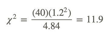
Therefore, since 11.9 is less than 55.758 (the value from the chi-square table given an alpha level of 0.05 and 40 degrees of freedom), we fail to reject the null hypothesis and, therefore, cannot conclude that the female gymnasts have a significantly higher variance in height than the general female high school population.
Calculating a Confidence Interval for a Population Variance
Once we know how to test a hypothesis about a single variance, calculating a confidence interval for a population variance is relatively easy. Again, it is important to remember that this test is dependent on the normality of the population. For non-normal populations, it is best to use the ANOVA test, which we will cover in greater detail in another lesson. To construct a confidence interval for the population variance, we need three pieces of information: the number of observations in the sample, the variance of the sample, and the desired confidence interval. With the desired confidence interval, α (most often this is set at 0.10 to reflect a 90% confidence interval or at 0.05 to reflect a 95% confidence interval), we can construct the upper and lower limits around the significance level.
Constructing a Confidence Interval
1. We randomly select 30 containers of Coca Cola and measure the amount of sugar in each container. Using the formula that we learned earlier, we calculate the variance of the sample to be 5.20. Find a 90% confidence interval for the true variance. In other words, assuming that the sample comes from a normal population, what is the range of the population variance?
To construct this 90% confidence interval, we first need to determine our upper and lower limits. The formula to construct this confidence interval and calculate the population variance, σ2, is as follows:
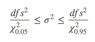
Using our standard chi-square distribution table, we can look up the critical χ2 values for 0.05 and 0.95 at 29 degrees of freedom. According to the χ2 distribution table, we find that χ20.05=42.557 and that χ20.95=17.708. Since we know the number of observations and the standard deviation for this sample, we can then solve for σ2 as shown below:
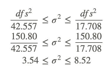
In other words, we are 90% confident that the variance of the population from which this sample was taken is between 3.54 and 8.52.
2. Assume the following data is from a normal population. Construct a 95% confidence interval for the standard deviation.
68.7 27.4 26 60.5 34.6 61.1 68.6 48.4 43.6 39.5 85.3 26.3 43.4 83.7 68.9
First, we need to find the sample standard deviation. This is easy enough to do by entering the data into a list and then use one variable statistics commands on a graphing calculator to determine the sample standard deviation, which you will find to be equal to 20.1. Note that there are 15 data points so the chi-square will have 14 degrees of freedom.
Next we have to find the formula for a confidence interval of the standard deviation, based off of the one for the variance:
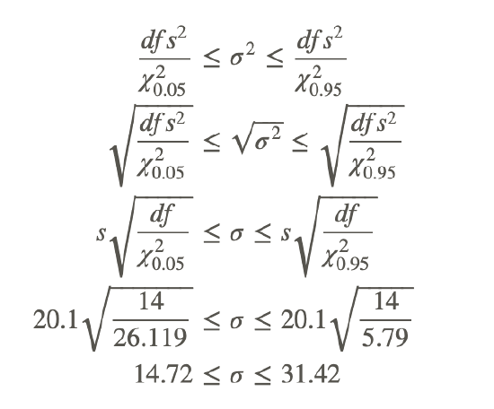
We believe that the population standard deviation is between 14.72 and 31.42.
Example
Example 1
Suppose a random sample of twenty boxes of crackers has a mean weight of 7.45 grams and a standard deviation of 4.1 grams. Assume the population is normally distributed. Find a 95% confidence interval for the standard deviation of the population.
Use the formula we derived in example C to find the confidence interval for the standard deviation:
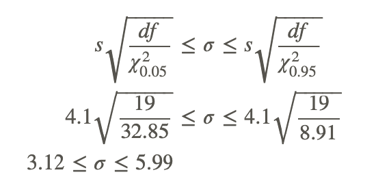
We are 95% confident that the population standard deviation is between 3.12 and 5.99.
Review
- We use the chi-square distribution for the:
- goodness-of-fit test
- test for independence
- testing of a hypothesis of single variance
- all of the above
- True or False: We can test a hypothesis about a single variance using the chi-square distribution for a non-normal population.
- In testing variance around the population mean, our null hypothesis states that the two population means that we are testing are:
- equal with respect to variance
- not equal
- none of the above
- In the formula for calculating the chi-square statistic for single variance, σ2 is:
- standard deviation
- number of observations
- hypothesized population variance
- chi-square statistic
- If we knew the number of observations in a sample, the standard deviation of the sample, and the hypothesized variance of the population, what additional information would we need to solve for the chi-square statistic?
- the chi-square distribution table
- the population size
- the standard deviation of the population
- no additional information is needed
- We want to test a hypothesis about a single variance using the chi-square distribution. We weighed 30 bars of Dial soap, and this sample had a standard deviation of 1.1. We want to test if this sample comes from the general factory, which we know from a previous study to have an overall variance of 3.22. What is our null hypothesis?
- Compute χ2 for Question 6.
- Given the information in Questions 6 and 7, would you reject or fail to reject the null hypothesis?
- Let’s assume that our population variance for this problem is unknown. We want to construct a 90% confidence interval around the population variance, σ2. If our critical values at a 90% confidence interval are 17.71 and 42.56, what is the range for σ2?
- What statement would you give surrounding this confidence interval?
- Consider the population mean and variance to be unknown. A random sample of size 8 is taken from a normal distribution. The sample has a variance of 0.64. A statistician is interested in testing the hypothesis: σ2=0.36 at the α=0.05 level. What is the result of this test? Explain.
- What is the p-value for the test in problem 11?
- Find a 90% confidence interval for the situation in problem 11.
- For a confidence interval for the population variance find the upper and lower critical values for a 95% confidence interval with ten degrees of freedom.
- A random sample of the population of 17 US state capitals has a mean of 330,731 and a standard deviation of 371,691. Assume that the population is normally distributed. Find a 90% confidence interval for the standard deviation of all US state capitals.
- For a random sample of size 25 and a sample variance of 12.2 what is the probability of observing a value this low or lower if, in fact, the true population variance is 15.4?
- Based on past experience a researcher believes the standard deviation of a population to be 12. A pilot study of n = 15 indicates a sample standard deviation of 9.25. At the 0.10 level of significance, what are the critical boundaries for rejecting H0:σ=12?
- A cereal company claims that their boxes of cereal weigh 15 ounces with a standard deviation of at most .5 ounces. Customers were complaining that this was not the case. The company needed to determine if the filling machine needed to be recalibrated. They took a sample of 84 boxes and determined that the standard deviation of their sample was 0.54. Does the machine need to be recalibrated?
- Does the cost of a graphing calculator vary from store to store? To answer this question a survey was taken of 43 stores. This survey yielded a sample mean of $84 and a sample standard deviation of $13. Test the claim that the standard deviation is greater than $15.
- Given the following survey data.
| Number of births | Frequency |
|---|---|
| 0 | 5 |
| 1 | 30 |
| 2 | 10 |
| 3 | 5 |
Does this data indicate that the population standard deviation is greater than 0.75?
- In a statistical hypothesis test, s2 is the sample variance and σ2 is the population variance and n is the sample size. What is the formula for the chi-square test for a single variance?
- Suppose a company claims that on average the cell phone batteries they produce last 60 minutes with a standard deviation of 4 minutes. The company randomly selects 7 batteries. The standard deviation of these batteries is 6 minutes.
- What is the chi-square statistic for this test?
- What are the null and alternative hypotheses for this test?
- What is the decision? Explain.
- Suppose the cell phone battery company takes a new random sample of 7 batteries. What is the probability that the standard deviation in the new test would be greater than 6 minutes?
- A doctor’s records show that height of a random sample 25 infants at age 12 months to be 29.530 inches with a standard deviation of 1.0953 inches. Construct a 95 percent confidence interval for population variance.
Vocabulary
| Term | Definition |
|---|---|
| ANOVA | The Analysis Of Variance, popularly known as the ANOVA, can be used in cases where there are more than two groups. |
| chi-squared distribution | The distribution of the chi-square statistic is called the chi-square distribution. |
| chi-squared statistic | The chi-squared statistic (X^2) is used to evaluate how well a set of observed data fits a corresponding expected set. |
| confidence intervals | A confidence interval is the interval within which you expect to capture a specific value. The confidence interval width is dependent on the confidence level. |
| variance | A measure of the spread of the data set equal to the mean of the squared variations of each data value from the mean of the data set. |
Additional Resources
Video: Chi-Squared Test of Population Variance Example
Practice: Tests of Single Variance

