2.4.2: Inverses by Mapping
- Page ID
- 14471
\( \newcommand{\vecs}[1]{\overset { \scriptstyle \rightharpoonup} {\mathbf{#1}} } \)
\( \newcommand{\vecd}[1]{\overset{-\!-\!\rightharpoonup}{\vphantom{a}\smash {#1}}} \)
\( \newcommand{\dsum}{\displaystyle\sum\limits} \)
\( \newcommand{\dint}{\displaystyle\int\limits} \)
\( \newcommand{\dlim}{\displaystyle\lim\limits} \)
\( \newcommand{\id}{\mathrm{id}}\) \( \newcommand{\Span}{\mathrm{span}}\)
( \newcommand{\kernel}{\mathrm{null}\,}\) \( \newcommand{\range}{\mathrm{range}\,}\)
\( \newcommand{\RealPart}{\mathrm{Re}}\) \( \newcommand{\ImaginaryPart}{\mathrm{Im}}\)
\( \newcommand{\Argument}{\mathrm{Arg}}\) \( \newcommand{\norm}[1]{\| #1 \|}\)
\( \newcommand{\inner}[2]{\langle #1, #2 \rangle}\)
\( \newcommand{\Span}{\mathrm{span}}\)
\( \newcommand{\id}{\mathrm{id}}\)
\( \newcommand{\Span}{\mathrm{span}}\)
\( \newcommand{\kernel}{\mathrm{null}\,}\)
\( \newcommand{\range}{\mathrm{range}\,}\)
\( \newcommand{\RealPart}{\mathrm{Re}}\)
\( \newcommand{\ImaginaryPart}{\mathrm{Im}}\)
\( \newcommand{\Argument}{\mathrm{Arg}}\)
\( \newcommand{\norm}[1]{\| #1 \|}\)
\( \newcommand{\inner}[2]{\langle #1, #2 \rangle}\)
\( \newcommand{\Span}{\mathrm{span}}\) \( \newcommand{\AA}{\unicode[.8,0]{x212B}}\)
\( \newcommand{\vectorA}[1]{\vec{#1}} % arrow\)
\( \newcommand{\vectorAt}[1]{\vec{\text{#1}}} % arrow\)
\( \newcommand{\vectorB}[1]{\overset { \scriptstyle \rightharpoonup} {\mathbf{#1}} } \)
\( \newcommand{\vectorC}[1]{\textbf{#1}} \)
\( \newcommand{\vectorD}[1]{\overrightarrow{#1}} \)
\( \newcommand{\vectorDt}[1]{\overrightarrow{\text{#1}}} \)
\( \newcommand{\vectE}[1]{\overset{-\!-\!\rightharpoonup}{\vphantom{a}\smash{\mathbf {#1}}}} \)
\( \newcommand{\vecs}[1]{\overset { \scriptstyle \rightharpoonup} {\mathbf{#1}} } \)
\(\newcommand{\longvect}{\overrightarrow}\)
\( \newcommand{\vecd}[1]{\overset{-\!-\!\rightharpoonup}{\vphantom{a}\smash {#1}}} \)
\(\newcommand{\avec}{\mathbf a}\) \(\newcommand{\bvec}{\mathbf b}\) \(\newcommand{\cvec}{\mathbf c}\) \(\newcommand{\dvec}{\mathbf d}\) \(\newcommand{\dtil}{\widetilde{\mathbf d}}\) \(\newcommand{\evec}{\mathbf e}\) \(\newcommand{\fvec}{\mathbf f}\) \(\newcommand{\nvec}{\mathbf n}\) \(\newcommand{\pvec}{\mathbf p}\) \(\newcommand{\qvec}{\mathbf q}\) \(\newcommand{\svec}{\mathbf s}\) \(\newcommand{\tvec}{\mathbf t}\) \(\newcommand{\uvec}{\mathbf u}\) \(\newcommand{\vvec}{\mathbf v}\) \(\newcommand{\wvec}{\mathbf w}\) \(\newcommand{\xvec}{\mathbf x}\) \(\newcommand{\yvec}{\mathbf y}\) \(\newcommand{\zvec}{\mathbf z}\) \(\newcommand{\rvec}{\mathbf r}\) \(\newcommand{\mvec}{\mathbf m}\) \(\newcommand{\zerovec}{\mathbf 0}\) \(\newcommand{\onevec}{\mathbf 1}\) \(\newcommand{\real}{\mathbb R}\) \(\newcommand{\twovec}[2]{\left[\begin{array}{r}#1 \\ #2 \end{array}\right]}\) \(\newcommand{\ctwovec}[2]{\left[\begin{array}{c}#1 \\ #2 \end{array}\right]}\) \(\newcommand{\threevec}[3]{\left[\begin{array}{r}#1 \\ #2 \\ #3 \end{array}\right]}\) \(\newcommand{\cthreevec}[3]{\left[\begin{array}{c}#1 \\ #2 \\ #3 \end{array}\right]}\) \(\newcommand{\fourvec}[4]{\left[\begin{array}{r}#1 \\ #2 \\ #3 \\ #4 \end{array}\right]}\) \(\newcommand{\cfourvec}[4]{\left[\begin{array}{c}#1 \\ #2 \\ #3 \\ #4 \end{array}\right]}\) \(\newcommand{\fivevec}[5]{\left[\begin{array}{r}#1 \\ #2 \\ #3 \\ #4 \\ #5 \\ \end{array}\right]}\) \(\newcommand{\cfivevec}[5]{\left[\begin{array}{c}#1 \\ #2 \\ #3 \\ #4 \\ #5 \\ \end{array}\right]}\) \(\newcommand{\mattwo}[4]{\left[\begin{array}{rr}#1 \amp #2 \\ #3 \amp #4 \\ \end{array}\right]}\) \(\newcommand{\laspan}[1]{\text{Span}\{#1\}}\) \(\newcommand{\bcal}{\cal B}\) \(\newcommand{\ccal}{\cal C}\) \(\newcommand{\scal}{\cal S}\) \(\newcommand{\wcal}{\cal W}\) \(\newcommand{\ecal}{\cal E}\) \(\newcommand{\coords}[2]{\left\{#1\right\}_{#2}}\) \(\newcommand{\gray}[1]{\color{gray}{#1}}\) \(\newcommand{\lgray}[1]{\color{lightgray}{#1}}\) \(\newcommand{\rank}{\operatorname{rank}}\) \(\newcommand{\row}{\text{Row}}\) \(\newcommand{\col}{\text{Col}}\) \(\renewcommand{\row}{\text{Row}}\) \(\newcommand{\nul}{\text{Nul}}\) \(\newcommand{\var}{\text{Var}}\) \(\newcommand{\corr}{\text{corr}}\) \(\newcommand{\len}[1]{\left|#1\right|}\) \(\newcommand{\bbar}{\overline{\bvec}}\) \(\newcommand{\bhat}{\widehat{\bvec}}\) \(\newcommand{\bperp}{\bvec^\perp}\) \(\newcommand{\xhat}{\widehat{\xvec}}\) \(\newcommand{\vhat}{\widehat{\vvec}}\) \(\newcommand{\uhat}{\widehat{\uvec}}\) \(\newcommand{\what}{\widehat{\wvec}}\) \(\newcommand{\Sighat}{\widehat{\Sigma}}\) \(\newcommand{\lt}{<}\) \(\newcommand{\gt}{>}\) \(\newcommand{\amp}{&}\) \(\definecolor{fillinmathshade}{gray}{0.9}\)Reflect points from \(f(x)\) across the line \(y = x\).
Your instructor gives you a function, \(f(x)=(x−1)^2+3\), where \(x\geq 1\), and asks you to find the inverse. You are all set to start manipulating the equation, when your Instructor specifies that you should find the inverse by graphing instead of by algebraic manipulation.
Are you able to do this?
Finding the Inverse by Mapping
Determining an inverse function algebraically can be both involved and difficult, so it is useful to know how to map \(f\) to \(f^{−1}\).
The graph of f can be used to produce the graph of \(f^{−1}\) by applying the inverse reflection principle:
The points \((a,b)\) and \((b,a)\) in the coordinate plane are symmetric with respect to the line \(y=x\).
The points \((a,b)\) and \((b,a)\) are reflections of each other across the line \(y=x\).
Finding the Inverse of a Function
1. Find the inverse of \(f(x)=\dfrac{1}{x−5}\) by mapping.
From the last section, we know that the inverse of this function is \(y=\dfrac{5x+1}{x}\). To find the inverse by mapping, pick several points on \(f(x)\), reflect them using the reflection principle and plot. Note: The coordinates of some of the points are rounded.
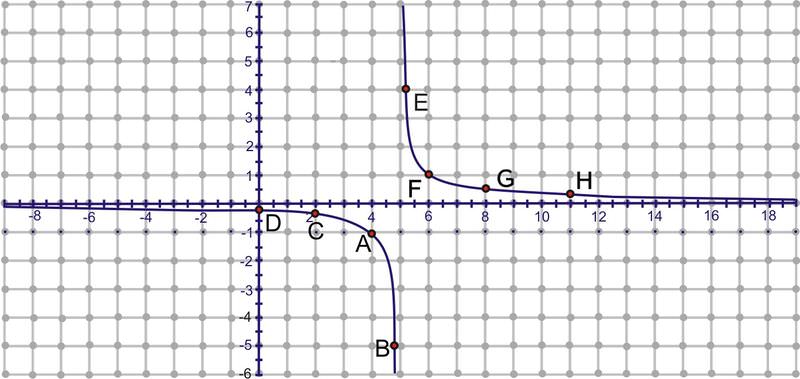
\(A: (4, -1)\)
\(B: (4.8, -5)\)
\(C: (2, -0.3)\)
\(D: (0, -0.2)\)
\(E: (5.3, 3.3)\)
\(F: (6, 1)\)
\(G: (8, 0.3)\)
\(H: (11, 0.2)\)
Now, take these eight points, switch the \(x\) and \(y\) and plot \((y,x)\). Connect them to make the inverse function.
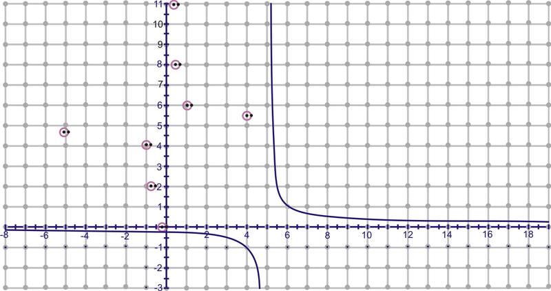
\(A^{−1}: (−1,4)\)
\(B^{−1}: (−5,4.8)\)
\(C^{−1}: (−0.3,2)\)
\(D^{−1}: (−0.2,0)\)
\(E^{−1}: (3.3,5.3)\)
\(F^{−1}: (1,6)\)
\(G^{−1}: (0.3,8)\)
\(H^{−1}: (0.2,11)\)
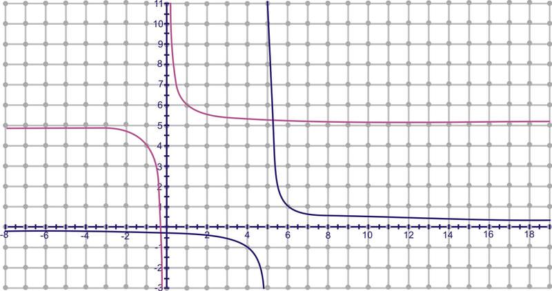
Not all functions have inverses that are one-to-one. However, the inverse can be modified to a one-to-one function if a “restricted domain” is applied to the inverse function.
2. Find the inverse of \(f(x)=x^2−4\).
Let’s use the graphic approach for this one. The function is graphed in blue and its inverse is red.
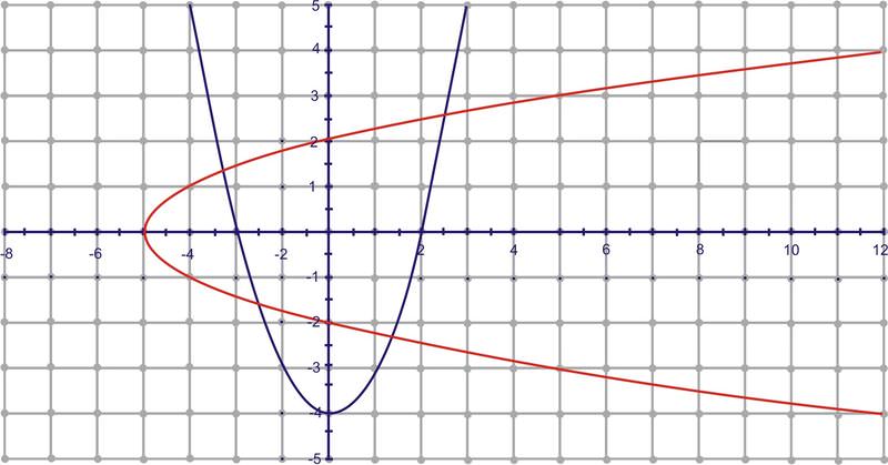
Clearly, the inverse relation is not a function because it does not pass the vertical line test. This is because all parabolas fail the horizontal line test. To “make” the inverse a function, we restrict the domain of the original function. For parabolas, this is fairly simple. To find the inverse of this function algebraically, we get \(f^{−1}(x)=\sqrt{x+4}\). Technically, however, the inverse is \(\pm\sqrt{x+4}\) because the square root of any number could be positive or negative. So, the inverse of \(f(x)=x^2−4\) is both parts of the square root equation, \(\sqrt{x+4}\) and \(−\sqrt{x+4}\). \(\sqrt{x+4}\) will yield the top portion of the horizontal parabola and \(−\sqrt{x+4}\) will yield the bottom half. Be careful, because if you just graph \(f^{−1}(x)=\sqrt{x+4}\) in your graphing calculator, it will only graph the top portion of the inverse.
This technique of sectioning the inverse is applied to finding the inverse of trigonometric functions because it is periodic.
3. Find the inverse of \(f(x)=\dfrac{x−1}{3x+2}\) mapping.
To find the inverse by mapping, pick several points on \(f(x)\), reflect them using the reflection principle and plot. Note: The coordinates of some of the points are rounded.
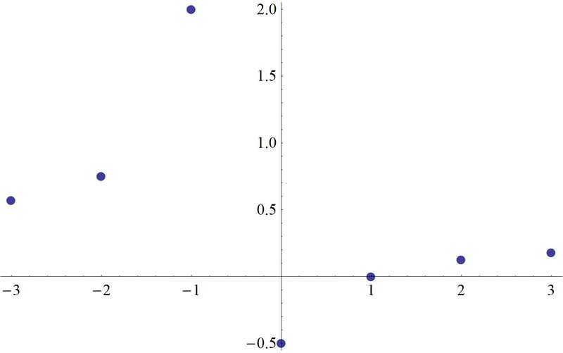
\(A: (0, -.5)\)
\(B: (-1, 2)\)
\(C: (1, 0)\)
\(D: (-2, .75)\)
\(E: (2, .125)\)
\(F: (-3, .57)\)
\(G: (3, .18)\)
Now, take these seven points, switch the \(x\) and \(y\) and plot \((y,x)\). Connect them to make the inverse function.
\(A^{−1}: (−.5,0)\)\)
\(B^{−1}: (2,−1)\)
\(C^{−1}: (0,1)\)
\(D^{−1}: (.75,−2)\)
\(E^{−1}: (.125,2)\)
\(F^{−1}: (.57,−3)\)
\(G^{−1}: (.18,3)\)
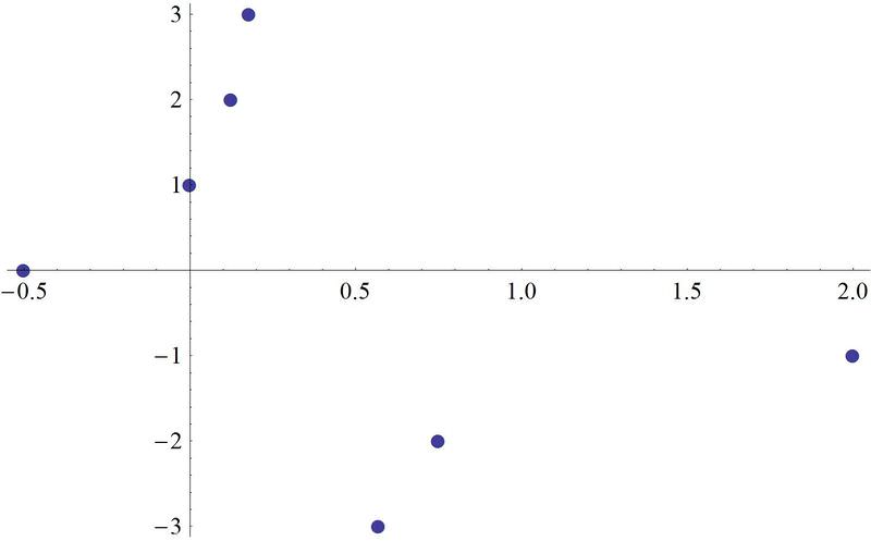
Not all functions have inverses that are one-to-one. However, the inverse can be modified to a one-to-one function if a “restricted domain” is applied to the inverse function.
Earlier, you were asked to find the inverse of a function.
The original equation is \(f(x)=(x−1)^2+3\).
Solution
Here is a plot of the function:
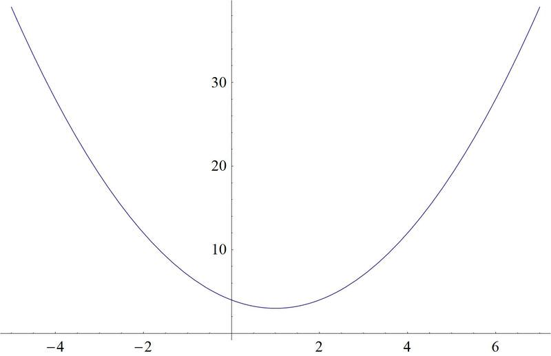
Notice that the domain of the function under examination has to be restricted to 1 or greater, so that the function will pass the horizontal line test. Some points that are on this graph are:
\(A: (1, 3)\)
\(B: (2, 4)\)
\(C: (3, 7)\)
To map the inverse function, first take each point and switch the "\(x\)" and "\(y\)" values:
\(A^{−1}: (3,1)\)
\(B^{−1}: (4,2)\)
\(C^{−1}: (7,3)\)
Then connect these dots, and you can see the graph of the inverse function. The inverse function graph looks like this:
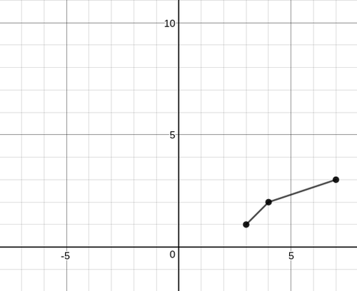
In this case, the range of the function has to be restricted to be 1 or greater, so that the inverse function will pass the vertical line test.
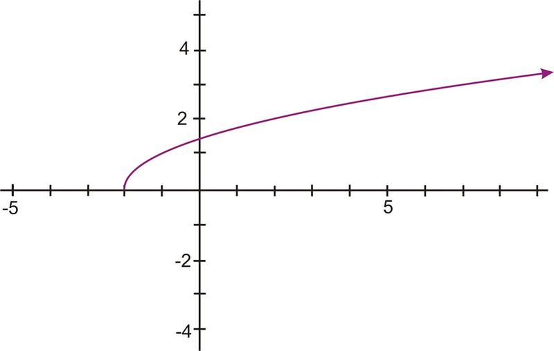
Study the following graph and answer these questions:
Is the graphed relation a function?
Does the relation have an inverse that is a function?
Solution
The graph represents a one-to-one function. It passes both a vertical and a horizontal line test. The inverse would be a function.
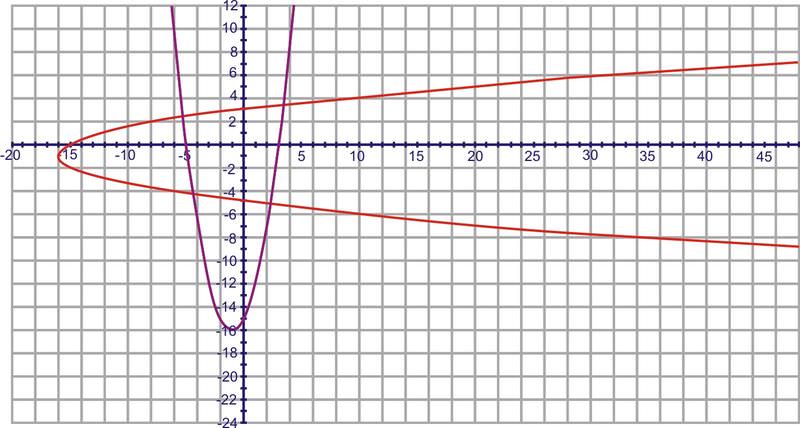
Find the inverse of \(f(x)=x^2+2x−15\) using the mapping principle.
Solution
By selecting 4-5 points and switching the \(x\) and \(y\) values, you will get the red graph below.
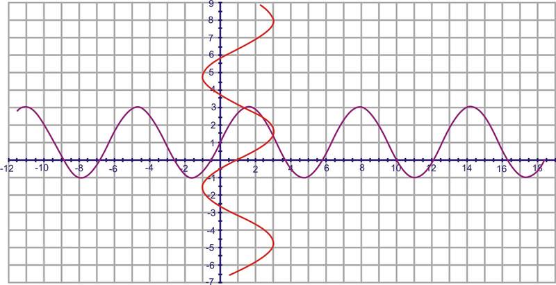
Find the inverse of \(y=1+2 \sin x\) using the mapping principle.
Solution
By selecting 4-5 points and switching the \(x\) and \(y\) values, you will get the red graph below.
Review
For each of the following graphs answer these questions:
(a) Is the graphed relation a function?
(b) Does the relation have an inverse that is a function?
-
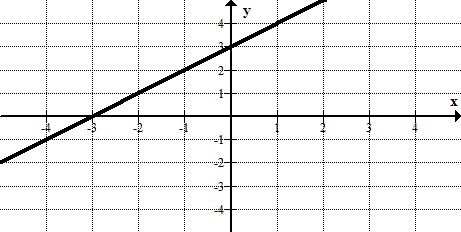
Figure \(\PageIndex{12}\) -
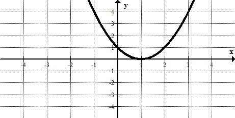
Figure \(\PageIndex{13}\) -
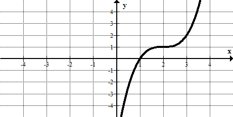
Figure \(\PageIndex{14}\) -
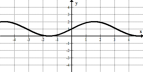
Figure \(\PageIndex{15}\) -
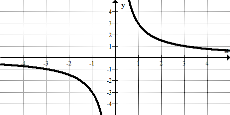
Figure \(\PageIndex{16}\) -
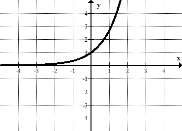
Figure \(\PageIndex{17}\)
Find the inverse of each function using the mapping principle.
- \(y=x^2+x−2\)
- \(y=x^3\)
- \(y=\sin\left (x−\dfrac{\pi}{2}\right)\)
- \(y=\cos(2x)\)
- \(y=\dfrac{1}{x}\)
- \(y=x^2−9\)
- \(y=−2+\sin\left(\dfrac{1}{2}x\right)\)
- What type of points will be in the same place in both a function and its inverse?
- When you graph a function and its inverse on the same set of axes, where is the line of reflection? Why?
Review (Answers)
To see the Review answers, open this PDF file and look for section 4.4.
Vocabulary
| Term | Definition |
|---|---|
| inverse function | Inverse functions are functions that 'undo' each other. Formally \(f(x)\) and \(g(x)\) are inverse functions if \(f(g(x))=g(f(x))=x\). |
| Mapping | Mapping is a procedure involving the plotting of points on a coordinate grid to see the behavior of a function. |

