2.6.6: Amplitude

Measure of a wave's height from the center axis.

The amplitude of the sine and cosine functions is the vertical distance between the sinusoidal axis and the maximum or minimum value of the function. In relation to sound waves, amplitude is a measure of how loud something is.

What is the most common mistake made when graphing the amplitude of a sine wave?

Amplitude of sinusoidal Functions

The general form a sinusoidal function is:

\(f(x)=\pm a\cdot \sin (b(x+c))+d\)

The cosine function can just as easily be substituted and for many problems it will be easier to use a cosine equation. since both the sine and cosine waves are identical except for a horizontal shift, it all depends on where you see the wave starting.

The coefficient a is the amplitude. When there is no number present, then the amplitude is 1. The best way to define amplitude is through a picture. Below is the graph of the function \(f(x)=3\cdot \sin x\), which has an amplitude of 3.

Figure \(\PageIndex{1}\)

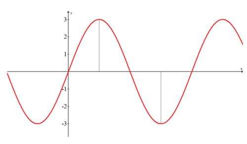
Notice that the amplitude is 3, not 6. This corresponds to the absolute value of the maximum and minimum values of the function. If the function had been \(f(x)=−3\cdot \sin x\), then the whole graph would be reflected across the x axis.

Also notice that the x axis on the graph above is unlabeled. This is to show that amplitude is a vertical distance. The sinusoidal axis is the neutral horizontal line that lies between the crests and the troughs (or peaks and valleys if you prefer). For this function, the sinusoidal axis was just the x axis, but if the whole graph were shifted up, the sinusoidal axis would no longer be the x axis. Instead, it would still be the horizontal line directly between the crests and troughs which is also the average of the maximum and minimum values.

Watch the portion of this video discussing amplitude:

Example \(\PageIndex{1}\)

Earlier, you were asked about the most common mistake made when graphing the amplitude of a singe wave. The most common mistake is doubling or halving the amplitude unnecessarily.

Solution

Earlier, you were asked about the most common mistake made when graphing the amplitude of a singe wave. The most common mistake is doubling or halving the amplitude unnecessarily.

Example \(\PageIndex{2}\)

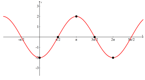
Graph the following function by plotting main points: \(f(x)=−2\cdot \cos x\).

Solution

The amplitude is 2, which means the maximum values will be at 2 and the minimum values will be at -2. Normally with a basic cosine curve the points corresponding to 0, \(\dfrac{\pi }{2}\), \(\pi\), \(\dfrac{3\pi }{2}\), \(2\pi \) fall above, on or below the line in the following sequence: above, on, below, on, above. The negative sign in the equation switches above with below and below with above. The whole graph is reflected across the x-axis.

Figure \(\PageIndex{2}\)

Example \(\PageIndex{3}\)

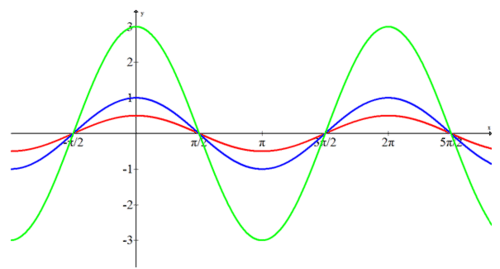
Write a cosine equation for each of the following functions.

Figure \(\PageIndex{3}\)

Solution

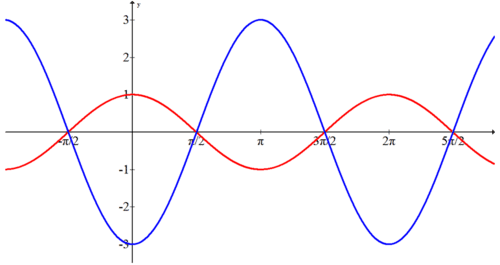
The amplitudes of the three functions are 3, 1 and \(\dfrac{1}{2}\) and none of them are reflected across the x-axis.

\(\begin{aligned} f(x)&=3\cdot \cos x \\ h(x)&=\cos x \\ g(x)&=\dfrac{1}{2}\cdot \cos x \end{aligned}\)

Note that amplitude itself is always positive.

Example \(\PageIndex{4}\)

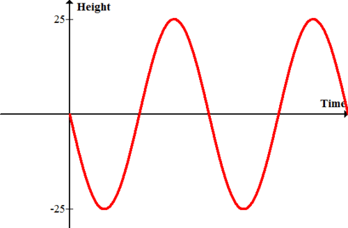
A Ferris wheel with radius 25 feet sits next to a platform. The ride starts at the platform and travels down to start. Model the height versus time of the ride.

Solution

since no information is given about the time, simply label the x axis as time. At time zero the height is zero. Initially the height will decrease as the ride goes below the platform. Eventually, the wheel will find the minimum and start to increase again all the way until it reaches a maximum.

Figure \(\PageIndex{4}\)

Example \(\PageIndex{5}\)

Find the amplitude of the function \(f(x)=−3\cos x\) and use the language of transformations to describe how the graph is related to the parent function \(y=\cos x\).

Solution

The new function is reflected across the x axis and vertically stretched by a factor of 3.

Figure \(\PageIndex{5}\)

Review

1. Explain how to find the amplitude of a sinusoidal function from its equation.
2. Explain how to find the amplitude of a sinusoidal function from its graph.

Find the amplitude of each of the following functions.

3. \(g(x)=−5\cos x\)

4. 

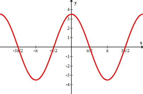
   Figure \(\PageIndex{6}\)

5. \(f(x)=\dfrac{1}{2} \sin x\)

6. 

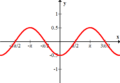
   Figure \(\PageIndex{7}\)

7. \(j(x)=3.12\cos x\)

8. 

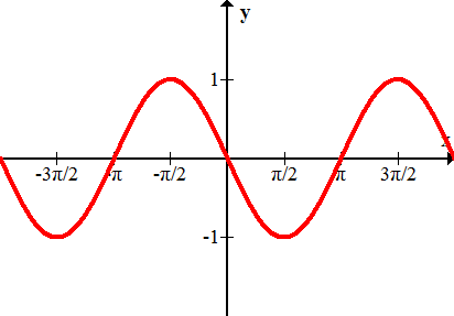
   Figure \(\PageIndex{8}\)

Sketch each of the following functions.

9. \(f(x)=3\sin x\)

10. \(g(x)=−4\cos x\)

11. \(h(x)=\pi \sin x\)

12. \(k(x)=−1.2\cos x\)

13. \(p(x)=\dfrac{2}{3} \cos x\)

14. \(m(x)=−\dfrac{1}{2} \sin x\)

15. Preview: \(r(x)=3\sin x+2\)

Review (Answers)

To see the Review answers, open this PDF file and look for section 5.3.

Additional Resources

Video: Amplitude and Period of sine and cosine