1.3.1: Limits and Asymptotes

Asymptotes and End Behavior

Most functions continue beyond the viewing window in our calculator or computer. People often draw an arrow next to a dotted line to indicate the pattern specifically. How can you recognize these asymptotes?

---

Asymptotes and End Behavior of Functions

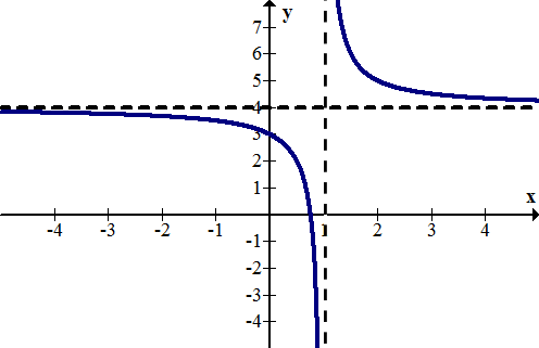
A vertical asymptote is a vertical line such as x=1 that indicates where a function is not defined and yet gets infinitely close to.

A horizontal asymptote is a horizontal line such as y=4 that indicates where a function flattens out as x gets very large or very small. A function may touch or pass through a horizontal asymptote.

The reciprocal function has two asymptotes, one vertical and one horizontal. Most computers and calculators do not draw the asymptotes and so they must be inserted by hand as dotted lines.

[Figure1]

Many students have the misconception that an asymptote is a line that a function gets infinitely close to but does not touch. This is not true. Take the following function:

[Figure2]

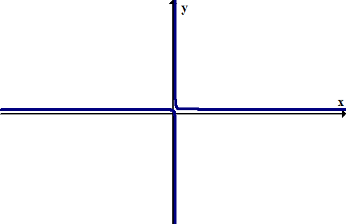
The graph appears to flatten as x grows larger. Thus, the horizontal asymptote is y=0 even though the function clearly passes through this line an infinite number of times.

The reason why asymptotes are important is because when your perspective is zoomed way out, the asymptotes essentially become the graph.

[Figure3]

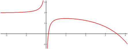
To find the asymptotes and end behavior of the function below, examine what happens to x and y as they each increase or decrease.

[Figure4]

The function has a horizontal asymptote y=2 as x approaches negative infinity. There is a vertical asymptote at x=0. The right hand side seems to decrease forever and has no asymptote.

Note that slant asymptotes do exist and are called oblique asymptotes.

---

Examples

Example 1

Solution

Earlier, you were asked how to identify asymptotes on a graph. Asymptotes written by hand are usually identified with dotted lines next to the function that indicate how the function will behave outside the viewing window. The equations of these vertical and horizontal dotted lines are of the form x=⎯⎯⎯⎯⎯⎯⎯⎯⎯⎯⎯ and y=⎯⎯⎯⎯⎯⎯⎯⎯⎯⎯⎯. When problems ask you to find the asymptotes of a function, they are asking for the equations of these horizontal and vertical lines.

Example 2

Identify the horizontal and vertical asymptotes of the following function.

[Figure5]

Solution

There is a vertical asymptote at x=0. As x gets infinitely small, there is a horizontal asymptote at y=−1. As x gets infinitely large, there is another horizontal asymptote at y=1.

Example 3

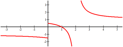
Identify the horizontal and vertical asymptotes of the following function.

[Figure6]

Solution

There is a vertical asymptote at x=2. As x gets infinitely small there is a horizontal asymptote at y=−1. As x gets infinitely large, there is a horizontal asymptote at y=1.

Example 4

Identify the horizontal and vertical asymptotes of the following piecewise function:

\(\ f(x)=\left\{\begin{array}{ll}
e^{x}-1 & x \leq 0 \\
\sin x & 0<x
\end{array}\right.\)

[Figure7]

Solution

There is a horizontal asymptote at y=−1 as x gets infinitely small. This is because e raised to the power of a very small number becomes 0.000000... and basically becomes zero.

Example 5

Identify the asymptotes and end behavior of the following function.

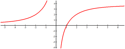[Figure8]

Solution

There is a vertical asymptote at x=0. The end behavior of the right and left side of this function does not match. The horizontal asymptote as x approaches negative infinity is y=0 and the horizontal asymptote as x approaches positive infinity is y=4. At this point you can only estimate these heights because you were not given the function or the tools to find these values analytically.

---

Review

Identify the asymptotes and end behavior of the following functions.

1. y=x

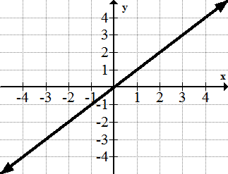[Figure9]

2. y=x²

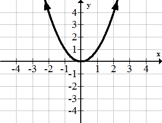[Figure10]

3. y=x³

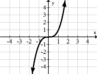[Figure11]

4. y=\(\ \sqrt{x}\)

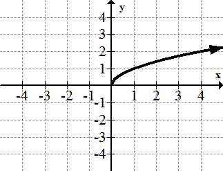[Figure12]

5. y= \(\ 1\over 2\)

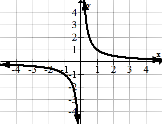[Figure13]

6. y=e^x

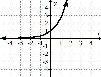[Figure14]

7. y=ln(x)

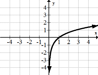[Figure15]

8. \(\ y=\frac{1}{1+e^{-x}}\)

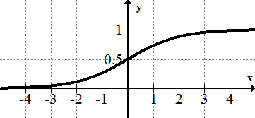[Figure16]

9.

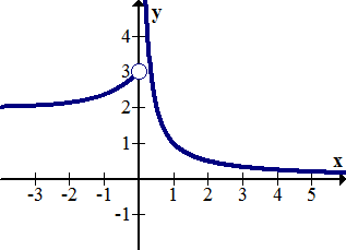[Figure17]

10.

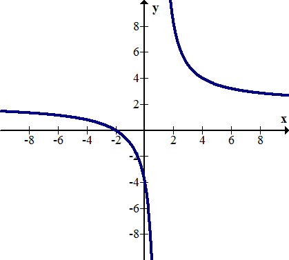[Figure18]

11.

[Figure19]

12. Vertical asymptotes occur at x values where a function is not defined. Explain why it makes sense that \(\ y=\frac{1}{x}\) has a vertical asymptote at x=0.

13. Vertical asymptotes occur at x values where a function is not defined. Explain why it makes sense that \(\ y=\frac{1}{x+3}\) has a vertical asymptote at x=−3.

14. Use the technique from the previous problem to determine the vertical asymptote for the function \(\ y=\frac{1}{x-2}\).

15. Use the technique from problem #13 to determine the vertical asymptote for the function \(\ y=\frac{2}{x+4}\)

---

Review (Answers)

To see the Review answers, open this PDF file and look for section 1.9.

---

Vocabulary

Term	Definition
Asymptotic	A function is asymptotic to a given line if the given line is an asymptote of the function.
Horizontal Asymptote	A horizontal asymptote is a horizontal line that indicates where a function flattens out as the independent variable gets very large or very small. A function may touch or pass through a horizontal asymptote.
Oblique Asymptote	An oblique asymptote is a diagonal line marking a specific range of values toward which the graph of a function may approach, but generally never reach. An oblique asymptote exists when the numerator of the function is exactly one degree greater than the denominator. An oblique asymptote may be found through long division.
Oblique Asymptotes	An oblique asymptote is a diagonal line marking a specific range of values toward which the graph of a function may approach, but generally never reach. An oblique asymptote exists when the numerator of the function is exactly one degree greater than the denominator. An oblique asymptote may be found through long division.
Piecewise Function	A piecewise function is a function that pieces together two or more parts of other functions to create a new function.
Slant Asymptote	A slant asymptote is a diagonal line marking a specific range of values toward which the graph of a function may approach, but will never reach. A slant asymptote exists when the numerator of the function is exactly one degree greater than the denominator. A slant asymptote may be found through long division.
Vertical Asymptote	A vertical asymptote is a vertical line marking a specific value toward which the graph of a function may approach, but will never reach.

---

Image Attributions

1. [Figure 1]
   Credit: CK-12 Foundation
   Source: https://commons.wikimedia.org/wiki/File:Boston_Police_Special_Operations_Unit.jpg
   License: CC BY-SA
2. [Figure 2]
   Credit: CK-12 Foundation
   License: CC BY-SA
3. [Figure 3]
   Credit: CK-12 Foundation
   License: CC BY-SA
4. [Figure 4]
   Credit: CK-12 Foundation
   License: CC BY-SA
5. [Figure 5]
   Credit: CK-12 Foundation
   Source: https://commons.wikimedia.org/wiki/File:Boston_Police_Special_Operations_Unit.jpg
   License: CC BY-SA
6. [Figure 6]
   Credit: CK-12 Foundation
   License: CC BY-SA
7. [Figure 7]
   Credit: CK-12 Foundation
   License: CC BY-SA
8. [Figure 8]
   Credit: CK-12 Foundation
   License: CC BY-SA
9. [Figure 9]
   Credit: CK-12 Foundation
   License: CC BY-SA
10. [Figure 10]
    Credit: CK-12 Foundation
    License: CC BY-SA
11. [Figure 11]
    Credit: CK-12 Foundation
    Source: http://classconnection.s3.amazonaws.com/753/flashcards/449753/png/screen_shot_2011-09-21_at_8.07.32_pm1316650094429.png
    License: CC BY-SA
12. [Figure 12]
    Credit: CK-12 Foundation
    License: CC BY-SA
13. [Figure 13]
    Credit: CK-12 Foundation
    License: CC BY-SA
14. [Figure 14]
    Credit: CK-12 Foundation
    License: CC BY-SA
15. [Figure 15]
    Credit: CK-12 Foundation
    License: CC BY-SA
16. [Figure 16]
    Credit: CK-12 Foundation;Paula Evans;Rob Young
    Source: https://www.flickr.com/photos/rob-young/1149735229/;https://commons.wikimedia.org/wiki/File:Will_%26_Grace_Apartment_Building_(1149735229).jpg
    License: CC BY-SA; CC BY-NC-SA
17. [Figure 17]
    Credit: CK-12 Foundation
    License: CC BY-SA
18. [Figure 18]
    Credit: CK-12 Foundation
    License: CC BY-SA
19. [Figure 19]
    Credit: CK-12 Foundation
    License: CC BY-SA