1.3.2: Infinite and Non-Existent Limits
- Page ID
- 14133
\( \newcommand{\vecs}[1]{\overset { \scriptstyle \rightharpoonup} {\mathbf{#1}} } \)
\( \newcommand{\vecd}[1]{\overset{-\!-\!\rightharpoonup}{\vphantom{a}\smash {#1}}} \)
\( \newcommand{\dsum}{\displaystyle\sum\limits} \)
\( \newcommand{\dint}{\displaystyle\int\limits} \)
\( \newcommand{\dlim}{\displaystyle\lim\limits} \)
\( \newcommand{\id}{\mathrm{id}}\) \( \newcommand{\Span}{\mathrm{span}}\)
( \newcommand{\kernel}{\mathrm{null}\,}\) \( \newcommand{\range}{\mathrm{range}\,}\)
\( \newcommand{\RealPart}{\mathrm{Re}}\) \( \newcommand{\ImaginaryPart}{\mathrm{Im}}\)
\( \newcommand{\Argument}{\mathrm{Arg}}\) \( \newcommand{\norm}[1]{\| #1 \|}\)
\( \newcommand{\inner}[2]{\langle #1, #2 \rangle}\)
\( \newcommand{\Span}{\mathrm{span}}\)
\( \newcommand{\id}{\mathrm{id}}\)
\( \newcommand{\Span}{\mathrm{span}}\)
\( \newcommand{\kernel}{\mathrm{null}\,}\)
\( \newcommand{\range}{\mathrm{range}\,}\)
\( \newcommand{\RealPart}{\mathrm{Re}}\)
\( \newcommand{\ImaginaryPart}{\mathrm{Im}}\)
\( \newcommand{\Argument}{\mathrm{Arg}}\)
\( \newcommand{\norm}[1]{\| #1 \|}\)
\( \newcommand{\inner}[2]{\langle #1, #2 \rangle}\)
\( \newcommand{\Span}{\mathrm{span}}\) \( \newcommand{\AA}{\unicode[.8,0]{x212B}}\)
\( \newcommand{\vectorA}[1]{\vec{#1}} % arrow\)
\( \newcommand{\vectorAt}[1]{\vec{\text{#1}}} % arrow\)
\( \newcommand{\vectorB}[1]{\overset { \scriptstyle \rightharpoonup} {\mathbf{#1}} } \)
\( \newcommand{\vectorC}[1]{\textbf{#1}} \)
\( \newcommand{\vectorD}[1]{\overrightarrow{#1}} \)
\( \newcommand{\vectorDt}[1]{\overrightarrow{\text{#1}}} \)
\( \newcommand{\vectE}[1]{\overset{-\!-\!\rightharpoonup}{\vphantom{a}\smash{\mathbf {#1}}}} \)
\( \newcommand{\vecs}[1]{\overset { \scriptstyle \rightharpoonup} {\mathbf{#1}} } \)
\(\newcommand{\longvect}{\overrightarrow}\)
\( \newcommand{\vecd}[1]{\overset{-\!-\!\rightharpoonup}{\vphantom{a}\smash {#1}}} \)
\(\newcommand{\avec}{\mathbf a}\) \(\newcommand{\bvec}{\mathbf b}\) \(\newcommand{\cvec}{\mathbf c}\) \(\newcommand{\dvec}{\mathbf d}\) \(\newcommand{\dtil}{\widetilde{\mathbf d}}\) \(\newcommand{\evec}{\mathbf e}\) \(\newcommand{\fvec}{\mathbf f}\) \(\newcommand{\nvec}{\mathbf n}\) \(\newcommand{\pvec}{\mathbf p}\) \(\newcommand{\qvec}{\mathbf q}\) \(\newcommand{\svec}{\mathbf s}\) \(\newcommand{\tvec}{\mathbf t}\) \(\newcommand{\uvec}{\mathbf u}\) \(\newcommand{\vvec}{\mathbf v}\) \(\newcommand{\wvec}{\mathbf w}\) \(\newcommand{\xvec}{\mathbf x}\) \(\newcommand{\yvec}{\mathbf y}\) \(\newcommand{\zvec}{\mathbf z}\) \(\newcommand{\rvec}{\mathbf r}\) \(\newcommand{\mvec}{\mathbf m}\) \(\newcommand{\zerovec}{\mathbf 0}\) \(\newcommand{\onevec}{\mathbf 1}\) \(\newcommand{\real}{\mathbb R}\) \(\newcommand{\twovec}[2]{\left[\begin{array}{r}#1 \\ #2 \end{array}\right]}\) \(\newcommand{\ctwovec}[2]{\left[\begin{array}{c}#1 \\ #2 \end{array}\right]}\) \(\newcommand{\threevec}[3]{\left[\begin{array}{r}#1 \\ #2 \\ #3 \end{array}\right]}\) \(\newcommand{\cthreevec}[3]{\left[\begin{array}{c}#1 \\ #2 \\ #3 \end{array}\right]}\) \(\newcommand{\fourvec}[4]{\left[\begin{array}{r}#1 \\ #2 \\ #3 \\ #4 \end{array}\right]}\) \(\newcommand{\cfourvec}[4]{\left[\begin{array}{c}#1 \\ #2 \\ #3 \\ #4 \end{array}\right]}\) \(\newcommand{\fivevec}[5]{\left[\begin{array}{r}#1 \\ #2 \\ #3 \\ #4 \\ #5 \\ \end{array}\right]}\) \(\newcommand{\cfivevec}[5]{\left[\begin{array}{c}#1 \\ #2 \\ #3 \\ #4 \\ #5 \\ \end{array}\right]}\) \(\newcommand{\mattwo}[4]{\left[\begin{array}{rr}#1 \amp #2 \\ #3 \amp #4 \\ \end{array}\right]}\) \(\newcommand{\laspan}[1]{\text{Span}\{#1\}}\) \(\newcommand{\bcal}{\cal B}\) \(\newcommand{\ccal}{\cal C}\) \(\newcommand{\scal}{\cal S}\) \(\newcommand{\wcal}{\cal W}\) \(\newcommand{\ecal}{\cal E}\) \(\newcommand{\coords}[2]{\left\{#1\right\}_{#2}}\) \(\newcommand{\gray}[1]{\color{gray}{#1}}\) \(\newcommand{\lgray}[1]{\color{lightgray}{#1}}\) \(\newcommand{\rank}{\operatorname{rank}}\) \(\newcommand{\row}{\text{Row}}\) \(\newcommand{\col}{\text{Col}}\) \(\renewcommand{\row}{\text{Row}}\) \(\newcommand{\nul}{\text{Nul}}\) \(\newcommand{\var}{\text{Var}}\) \(\newcommand{\corr}{\text{corr}}\) \(\newcommand{\len}[1]{\left|#1\right|}\) \(\newcommand{\bbar}{\overline{\bvec}}\) \(\newcommand{\bhat}{\widehat{\bvec}}\) \(\newcommand{\bperp}{\bvec^\perp}\) \(\newcommand{\xhat}{\widehat{\xvec}}\) \(\newcommand{\vhat}{\widehat{\vvec}}\) \(\newcommand{\uhat}{\widehat{\uvec}}\) \(\newcommand{\what}{\widehat{\wvec}}\) \(\newcommand{\Sighat}{\widehat{\Sigma}}\) \(\newcommand{\lt}{<}\) \(\newcommand{\gt}{>}\) \(\newcommand{\amp}{&}\) \(\definecolor{fillinmathshade}{gray}{0.9}\)Infinite and Non-Existent Limits
You have heard time and again that it is "against the rules" to divide by the number 0. Even the most basic calculator will return some form of "ERROR" if you try to divide even the smallest of numbers by 0.
Do you really understand why it is "against the rules"? What is really wrong with dividing by nothing?
Infinite and Non-Existent Limits
Functions can exhibit a number of different behaviors as the input value gets very large or very small.
As x approaches ∞, some functions output values get closer and closer to a single number, some approach zero, and some continue to get larger and larger or smaller and smaller without limit.
In this lesson, we will explore functions of the last type, functions with infinite limits, and the different types of asymptotes they may have.
Examples
Solution
Earlier, you were given a question about dividing by zero.
Dividing by zero is "against the rules" because there is no definition for the answer you would get.
Consider what happens as you take a given value and divide it by smaller and smaller numbers:
- 2 / 10 = 1/5
- 2 / 1 = 2
- 2 / .1 = 20
- 2 / .001 = 2,000
- 2 / .000000001 = 2,000,000,000
As we divide by progressively smaller numbers, the quotient gets larger and larger. Also, we can see that in each case, the problem could be reversed by multiplying the product by the dividend to get the divisor, for instance: 2 / .1 = 20 ==> 20 * .1 = 2.
Unfortunately, this doesn't work if you actually divide by 0, even if you assume that dividing by zero resulted in infinity! No matter how big the number you multiply by zero, even infinity, you will never be able to get back to 2.
\(\ \therefore \frac{x}{0}=\text { undefined }\)
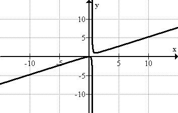
Evaluate the function \(\ h(x)=\frac{x^{2}}{2 x-1}\)

Solution
To evaluate this function, consider the behavior of the function as larger and larger values are inserted for x. As x approaches ∞, the function values also approach ∞. Therefore the limit of the function as x approaches ∞ is: \(\ \lim _{x \rightarrow \infty} \frac{x^{2}}{2 x-1}=\infty\). Similarly, as x approaches −∞, f(x) approaches −∞. Therefore we have \(\ \lim _{x \rightarrow-\infty} \frac{x^{2}}{2 x-1}=-\infty\).
We can also understand this limit if we analyze the equation for h(x). As x gets larger and larger, the value of the expression 2x - 1 gets closer and closer to the value of the expression 2x. That is, for sufficiently large values of x, 2x - 1 ≈ 2x. Therefore the values of h(x) approach \(\ \frac{x^{2}}{2 x}=\frac{x}{2}\).
As x gets larger and larger, so does \(\ x\over 2\). For large values of x, the function h(x) gets closer and closer to \(\ x\over 2\). Therefore the limit is infinity.
Approximate the function f(x) = x2 + 2x - 3.
Solution
This function has an infinite limit as x approaches infinity. However, as x gets larger and larger, f(x) ≈ x2, since the x2 value grows much more quickly than the 2x value, particularly apparent at very large +/- values of x. If this is not immediately apparent, evaluate the function for x = 1,000,000, and you will quickly get the idea!
Therefore we can use the function y = x2 to describe the end behavior of f(x).
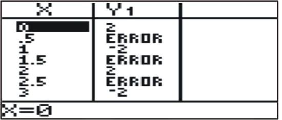
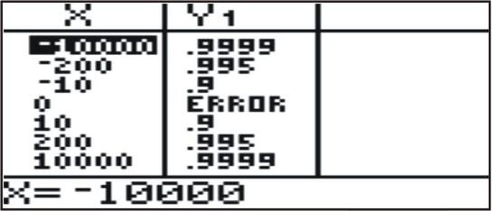
Describe the end behavior of each graph. That is, determine if the function has a limit L, if the limit is infinite, or if the limit does not exist.
- y=x2
- y=2(−1)x
- \(\ y=1-\frac{1}{|x|}\)
Solution
- As x approaches +∞, x2 also approaches +∞. As x approaches −∞, x2 approaches +∞. Therefore \(\ \lim _{x \rightarrow \infty} x^{2}=\lim _{x \rightarrow-\infty} x^{2}=\infty\).
- This function is difficult to understand without producing a graph. The table shows that the function only takes on two values: 2, and -2, and is undefined at non-integer values of x. As x approaches +∞ or −∞, the function values alternate between 2 and -2. Therefore the limit does not exist.

- If you look at the table of this function, which has negative and positive values of x, you can see that as x approaches +∞ or −∞, the function values approach 1.

Therefore \(\ \lim _{x \rightarrow \infty}\left(1-\frac{1}{|x|}\right)=\lim _{x \rightarrow-\infty}\left(1-\frac{1}{|x|}\right)=1\).
We can also determine this limit analytically. For large values of x, |x| is also large, and so \(\ \frac{1}{|x|}\) is small (since dividing 1 by a large number results in a very small number). Therefore, for large values of \(\ x, 1-\frac{1}{|x|} \approx 1-0=1\). We can make the same argument for x approaching −∞.
Evaluate \(\ \lim _{x \rightarrow \infty} \frac{x^{2}+2 x}{x-3}\).
Solution
The numerator is of greater degree than the denominator, so the function does not approach a limit. The denominator is x - 3, so the graph cannot include 3.
Evaluate −2x3−5x2+8x.
Solution
−2x3−5x2+8x is a 3rd degree equation, so it will turn twice, since it is not a rational function, there are no concerns about numerator or denominator. The function will have no limits, and will grow without bound in both the positive and negative directions. If you use a graphing calculator to graph the function, you will see that y=x3 can be used to approximate it.
Review
For questions 1-3: The limit of f(x) as x→t cannot exist if which conditions are true? List three conditions.
- One condition is...
- A second condition is...
- A third condition is...
- Give an example of a limit that does not exist
Questions 5-7: Assuming that f(x) is a rational function:
- What is \(\ \lim _{x \rightarrow \infty} f(x)\) when the degree of the numerator is less than the degree of the denominator?
- What is \(\ \lim _{x \rightarrow \infty} f(x)\) when the degrees of the numerator and the denominator are equal?
- What is \(\ \lim _{x \rightarrow \infty} f(x)\) when the degree of the numerator is greater than the degree of the denominator?
- In general, if r is a positive real number, what is \(\ \lim _{x \rightarrow \infty} \frac{1}{x^{r}}\)?
- In general, if r is a positive real number, what is \(\ \lim _{x \rightarrow \infty} x^{r}\)?
Questions 10-13: Let a and b be real numbers and let t be a positive integer. Complete each of the following properties of limits.
10. \(\ \lim _{x \rightarrow a} x^{t}=\)
11. If f is a polynomial, \(\ \lim _{x \rightarrow a} f(x)=\)
12. \(\ \lim _{x \rightarrow a} k \cdot f(x)=\)
13. \(\ \lim _{x \rightarrow \infty} t^{x}=\)
Questions 14-16: Evaluate.
14. \(\ \lim _{x \rightarrow-5} \frac{(5+x)^{2}-25}{x}\)
15. \(\ \lim _{x \rightarrow 3} \frac{x^{3}-6 x+2}{x^{2}+2 x-3}\)
16. \(\ \lim _{x \rightarrow 0} \frac{(3+3 y)^{-1}-3 y^{-1}}{x}\)
Vocabulary
| Term | Definition |
|---|---|
| ∞ | The symbol "∞" means "infinity", and is an abstract concept describing a value greater than any countable number. |
| Asymptotes | An asymptote is a line on the graph of a function representing a value toward which the function may approach, but does not reach (with certain exceptions). |
| infinite limit | A function has an infinite limit if it's output approaches infinity or negative infinity as very large or very small values are calculated for the input variable (usually "x"). |
| infinity | Infinity is an unbounded quantity that is greater than any countable number. The symbol for infinity is ∞. |
| limit | A limit is the value that the output of a function approaches as the input of the function approaches a given value. |

