2.4: Basic Trigonometric Limits
- Page ID
- 1115
\( \newcommand{\vecs}[1]{\overset { \scriptstyle \rightharpoonup} {\mathbf{#1}} } \)
\( \newcommand{\vecd}[1]{\overset{-\!-\!\rightharpoonup}{\vphantom{a}\smash {#1}}} \)
\( \newcommand{\id}{\mathrm{id}}\) \( \newcommand{\Span}{\mathrm{span}}\)
( \newcommand{\kernel}{\mathrm{null}\,}\) \( \newcommand{\range}{\mathrm{range}\,}\)
\( \newcommand{\RealPart}{\mathrm{Re}}\) \( \newcommand{\ImaginaryPart}{\mathrm{Im}}\)
\( \newcommand{\Argument}{\mathrm{Arg}}\) \( \newcommand{\norm}[1]{\| #1 \|}\)
\( \newcommand{\inner}[2]{\langle #1, #2 \rangle}\)
\( \newcommand{\Span}{\mathrm{span}}\)
\( \newcommand{\id}{\mathrm{id}}\)
\( \newcommand{\Span}{\mathrm{span}}\)
\( \newcommand{\kernel}{\mathrm{null}\,}\)
\( \newcommand{\range}{\mathrm{range}\,}\)
\( \newcommand{\RealPart}{\mathrm{Re}}\)
\( \newcommand{\ImaginaryPart}{\mathrm{Im}}\)
\( \newcommand{\Argument}{\mathrm{Arg}}\)
\( \newcommand{\norm}[1]{\| #1 \|}\)
\( \newcommand{\inner}[2]{\langle #1, #2 \rangle}\)
\( \newcommand{\Span}{\mathrm{span}}\) \( \newcommand{\AA}{\unicode[.8,0]{x212B}}\)
\( \newcommand{\vectorA}[1]{\vec{#1}} % arrow\)
\( \newcommand{\vectorAt}[1]{\vec{\text{#1}}} % arrow\)
\( \newcommand{\vectorB}[1]{\overset { \scriptstyle \rightharpoonup} {\mathbf{#1}} } \)
\( \newcommand{\vectorC}[1]{\textbf{#1}} \)
\( \newcommand{\vectorD}[1]{\overrightarrow{#1}} \)
\( \newcommand{\vectorDt}[1]{\overrightarrow{\text{#1}}} \)
\( \newcommand{\vectE}[1]{\overset{-\!-\!\rightharpoonup}{\vphantom{a}\smash{\mathbf {#1}}}} \)
\( \newcommand{\vecs}[1]{\overset { \scriptstyle \rightharpoonup} {\mathbf{#1}} } \)
\( \newcommand{\vecd}[1]{\overset{-\!-\!\rightharpoonup}{\vphantom{a}\smash {#1}}} \)
\(\newcommand{\avec}{\mathbf a}\) \(\newcommand{\bvec}{\mathbf b}\) \(\newcommand{\cvec}{\mathbf c}\) \(\newcommand{\dvec}{\mathbf d}\) \(\newcommand{\dtil}{\widetilde{\mathbf d}}\) \(\newcommand{\evec}{\mathbf e}\) \(\newcommand{\fvec}{\mathbf f}\) \(\newcommand{\nvec}{\mathbf n}\) \(\newcommand{\pvec}{\mathbf p}\) \(\newcommand{\qvec}{\mathbf q}\) \(\newcommand{\svec}{\mathbf s}\) \(\newcommand{\tvec}{\mathbf t}\) \(\newcommand{\uvec}{\mathbf u}\) \(\newcommand{\vvec}{\mathbf v}\) \(\newcommand{\wvec}{\mathbf w}\) \(\newcommand{\xvec}{\mathbf x}\) \(\newcommand{\yvec}{\mathbf y}\) \(\newcommand{\zvec}{\mathbf z}\) \(\newcommand{\rvec}{\mathbf r}\) \(\newcommand{\mvec}{\mathbf m}\) \(\newcommand{\zerovec}{\mathbf 0}\) \(\newcommand{\onevec}{\mathbf 1}\) \(\newcommand{\real}{\mathbb R}\) \(\newcommand{\twovec}[2]{\left[\begin{array}{r}#1 \\ #2 \end{array}\right]}\) \(\newcommand{\ctwovec}[2]{\left[\begin{array}{c}#1 \\ #2 \end{array}\right]}\) \(\newcommand{\threevec}[3]{\left[\begin{array}{r}#1 \\ #2 \\ #3 \end{array}\right]}\) \(\newcommand{\cthreevec}[3]{\left[\begin{array}{c}#1 \\ #2 \\ #3 \end{array}\right]}\) \(\newcommand{\fourvec}[4]{\left[\begin{array}{r}#1 \\ #2 \\ #3 \\ #4 \end{array}\right]}\) \(\newcommand{\cfourvec}[4]{\left[\begin{array}{c}#1 \\ #2 \\ #3 \\ #4 \end{array}\right]}\) \(\newcommand{\fivevec}[5]{\left[\begin{array}{r}#1 \\ #2 \\ #3 \\ #4 \\ #5 \\ \end{array}\right]}\) \(\newcommand{\cfivevec}[5]{\left[\begin{array}{c}#1 \\ #2 \\ #3 \\ #4 \\ #5 \\ \end{array}\right]}\) \(\newcommand{\mattwo}[4]{\left[\begin{array}{rr}#1 \amp #2 \\ #3 \amp #4 \\ \end{array}\right]}\) \(\newcommand{\laspan}[1]{\text{Span}\{#1\}}\) \(\newcommand{\bcal}{\cal B}\) \(\newcommand{\ccal}{\cal C}\) \(\newcommand{\scal}{\cal S}\) \(\newcommand{\wcal}{\cal W}\) \(\newcommand{\ecal}{\cal E}\) \(\newcommand{\coords}[2]{\left\{#1\right\}_{#2}}\) \(\newcommand{\gray}[1]{\color{gray}{#1}}\) \(\newcommand{\lgray}[1]{\color{lightgray}{#1}}\) \(\newcommand{\rank}{\operatorname{rank}}\) \(\newcommand{\row}{\text{Row}}\) \(\newcommand{\col}{\text{Col}}\) \(\renewcommand{\row}{\text{Row}}\) \(\newcommand{\nul}{\text{Nul}}\) \(\newcommand{\var}{\text{Var}}\) \(\newcommand{\corr}{\text{corr}}\) \(\newcommand{\len}[1]{\left|#1\right|}\) \(\newcommand{\bbar}{\overline{\bvec}}\) \(\newcommand{\bhat}{\widehat{\bvec}}\) \(\newcommand{\bperp}{\bvec^\perp}\) \(\newcommand{\xhat}{\widehat{\xvec}}\) \(\newcommand{\vhat}{\widehat{\vvec}}\) \(\newcommand{\uhat}{\widehat{\uvec}}\) \(\newcommand{\what}{\widehat{\wvec}}\) \(\newcommand{\Sighat}{\widehat{\Sigma}}\) \(\newcommand{\lt}{<}\) \(\newcommand{\gt}{>}\) \(\newcommand{\amp}{&}\) \(\definecolor{fillinmathshade}{gray}{0.9}\)Trigonometric functions can be a component of an expression and therefore subject to a limit process. Do you think that the periodic nature of these functions, and the limited or infinity range of individual trigonometric functions would make evaluating limits involving these functions difficult?
Limits with Trigonometric Functions
The limit rules presented in earlier concepts offer some, but not all, of the tools for evaluating limits involving trigonometric functions.
Let's find the following limits:
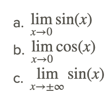
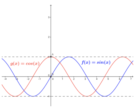
We can find these limits by evaluating the function as x approaches 0 on the left and the right, i.e., by evaluating the two one-sided limits. The graphs and tables values are shown below.
CC BY-NC-SA
| x(rad) |
-0.001 |
-0.0001 |
0 |
0.0001 |
0.001 |
|
sin(x) |
-0.001 |
-0.0001 |
0 |
0.0001 |
0.001 |
|
cos(x) |
0.999 |
0.9999 |
1 |
0.9999 |
0.999 |
Inspection of the graph below, and table of values in the vicinity of x=0, indicates that:

Note that the limits can be found using direct substitution.
- Because sin(x) is a periodic function, as x gets larger (smaller) and larger (smaller), its value will oscillate between 1 and -1, and never settle to a single value. Therefore, we can say that

does not exist.
We can generalize and extend the findings above and present the following properties:
Limit Properties for Basic Trigonometric Functions
- Limit as x→a for any real a:
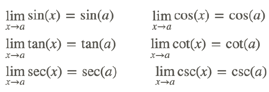
- Limit as x→±∞:

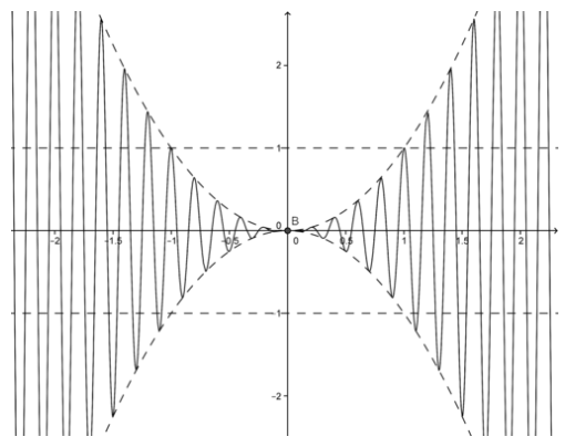
Let's find find

The graph of the function is shown below.
CC BY-NC-SA
Since we know that the limit of x2 and cos(x) exist, we can find the limit of this function by applying the Product Rule, or direct substitution:

Hence,

Also, from the graph of the function, we note that the function is bounded by the graphs of x2 and −x2, which both are 0 at x=0. It makes sense that the original function’s limit should be 0.
The Squeeze Theorem
This feature, that a function’s limit can result from the function being bounded or squeezed by two other functions, is the basis for the Squeeze Theorem. The Squeeze Theorem (also known as the Sandwich Theorem) states:

In other words, if we can find bounds for a function that have the same limit, then the limit of the function that they bound must have the same limit. Note that a and L may be any constant or even ∞ or −∞.
One of the important trigonometric limits that can be proved, in part, using the Squeeze Theorem is:
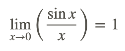
where x is in radian measure.
Another important trigonometric limit is
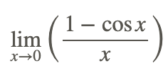
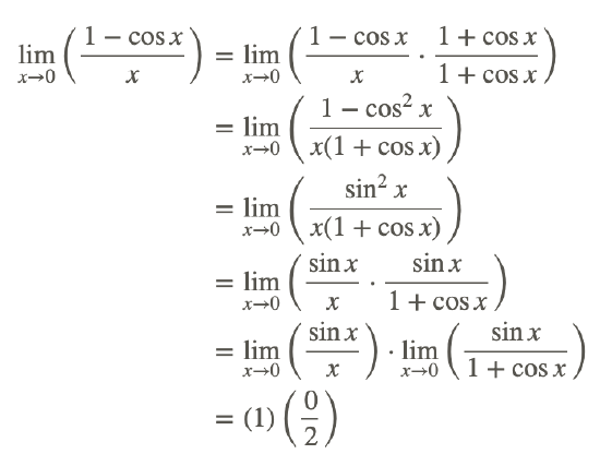
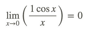
Direct substitution cannot be used to evaluate the limit because it yields the indeterminate form 0/0. Instead, transform the problem to a different form and solve.
Examples
Example 1
Earlier, you were asked if the periodic nature of trigonometric functions and the limited or infinity range of individual trigonometric functions make evaluating limits involving trigonometric functions difficult.
As you can imagine and have seen in this concept, some limits involving trigonometric functions can be easily evaluated by direct substitution, and some evolve a lot of work to change form from an indeterminate or undefined form. Determining the end behavior of an expression involving a trigonometric function can also be difficult, and require application of principles like the Squeeze Theorem to obtain a result. No easy answer!
Example 2
Find

Direct substitution cannot be used to evaluate the limit because 10π/x is undefined when x=0.
However, the Squeeze Theorem can be used as follows:
1. We know that cosine stays between -1 and 1, so

for any x in the domain of the function (i.e., any x≠0).
2. Since x2 is always non-negative, we can multiply the above inequality by x2:

3. The original function is bounded by x2 and −x2 and

4. Therefore, by the Squeeze Theorem:

Review
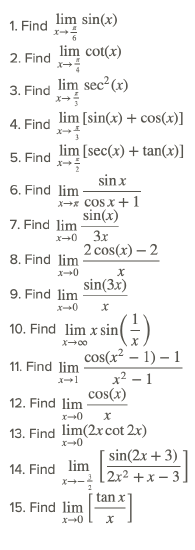
Vocabulary
| Term | Definition |
|---|---|
| indeterminate | In mathematics, an expression is indeterminate if it is not precisely defined. There are seven indeterminate forms: 00,0⋅∞,∞∞,∞−∞,00,∞0, and 1^\infty. |
| limit | A limit is the value that the output of a function approaches as the input of the function approaches a given value. |
| squeeze theorem | The squeeze theorem (also known as the sandwich theorem) is used to find the limit of a function by bounding it between two other functions that each have the same limit. |
Additional Resources
PLIX: Play, Learn, Interact, eXplore - Evaluating Limits of tan(x)
Video: Determining Limits Involving Trigonometric Functions
Practice: Basic Trigonometric Limits
Real World: I'll Fly Away

