3.3: Intermediate Value Theorem, Existence of Solution
- Page ID
- 1198
\( \newcommand{\vecs}[1]{\overset { \scriptstyle \rightharpoonup} {\mathbf{#1}} } \)
\( \newcommand{\vecd}[1]{\overset{-\!-\!\rightharpoonup}{\vphantom{a}\smash {#1}}} \)
\( \newcommand{\id}{\mathrm{id}}\) \( \newcommand{\Span}{\mathrm{span}}\)
( \newcommand{\kernel}{\mathrm{null}\,}\) \( \newcommand{\range}{\mathrm{range}\,}\)
\( \newcommand{\RealPart}{\mathrm{Re}}\) \( \newcommand{\ImaginaryPart}{\mathrm{Im}}\)
\( \newcommand{\Argument}{\mathrm{Arg}}\) \( \newcommand{\norm}[1]{\| #1 \|}\)
\( \newcommand{\inner}[2]{\langle #1, #2 \rangle}\)
\( \newcommand{\Span}{\mathrm{span}}\)
\( \newcommand{\id}{\mathrm{id}}\)
\( \newcommand{\Span}{\mathrm{span}}\)
\( \newcommand{\kernel}{\mathrm{null}\,}\)
\( \newcommand{\range}{\mathrm{range}\,}\)
\( \newcommand{\RealPart}{\mathrm{Re}}\)
\( \newcommand{\ImaginaryPart}{\mathrm{Im}}\)
\( \newcommand{\Argument}{\mathrm{Arg}}\)
\( \newcommand{\norm}[1]{\| #1 \|}\)
\( \newcommand{\inner}[2]{\langle #1, #2 \rangle}\)
\( \newcommand{\Span}{\mathrm{span}}\) \( \newcommand{\AA}{\unicode[.8,0]{x212B}}\)
\( \newcommand{\vectorA}[1]{\vec{#1}} % arrow\)
\( \newcommand{\vectorAt}[1]{\vec{\text{#1}}} % arrow\)
\( \newcommand{\vectorB}[1]{\overset { \scriptstyle \rightharpoonup} {\mathbf{#1}} } \)
\( \newcommand{\vectorC}[1]{\textbf{#1}} \)
\( \newcommand{\vectorD}[1]{\overrightarrow{#1}} \)
\( \newcommand{\vectorDt}[1]{\overrightarrow{\text{#1}}} \)
\( \newcommand{\vectE}[1]{\overset{-\!-\!\rightharpoonup}{\vphantom{a}\smash{\mathbf {#1}}}} \)
\( \newcommand{\vecs}[1]{\overset { \scriptstyle \rightharpoonup} {\mathbf{#1}} } \)
\( \newcommand{\vecd}[1]{\overset{-\!-\!\rightharpoonup}{\vphantom{a}\smash {#1}}} \)
\(\newcommand{\avec}{\mathbf a}\) \(\newcommand{\bvec}{\mathbf b}\) \(\newcommand{\cvec}{\mathbf c}\) \(\newcommand{\dvec}{\mathbf d}\) \(\newcommand{\dtil}{\widetilde{\mathbf d}}\) \(\newcommand{\evec}{\mathbf e}\) \(\newcommand{\fvec}{\mathbf f}\) \(\newcommand{\nvec}{\mathbf n}\) \(\newcommand{\pvec}{\mathbf p}\) \(\newcommand{\qvec}{\mathbf q}\) \(\newcommand{\svec}{\mathbf s}\) \(\newcommand{\tvec}{\mathbf t}\) \(\newcommand{\uvec}{\mathbf u}\) \(\newcommand{\vvec}{\mathbf v}\) \(\newcommand{\wvec}{\mathbf w}\) \(\newcommand{\xvec}{\mathbf x}\) \(\newcommand{\yvec}{\mathbf y}\) \(\newcommand{\zvec}{\mathbf z}\) \(\newcommand{\rvec}{\mathbf r}\) \(\newcommand{\mvec}{\mathbf m}\) \(\newcommand{\zerovec}{\mathbf 0}\) \(\newcommand{\onevec}{\mathbf 1}\) \(\newcommand{\real}{\mathbb R}\) \(\newcommand{\twovec}[2]{\left[\begin{array}{r}#1 \\ #2 \end{array}\right]}\) \(\newcommand{\ctwovec}[2]{\left[\begin{array}{c}#1 \\ #2 \end{array}\right]}\) \(\newcommand{\threevec}[3]{\left[\begin{array}{r}#1 \\ #2 \\ #3 \end{array}\right]}\) \(\newcommand{\cthreevec}[3]{\left[\begin{array}{c}#1 \\ #2 \\ #3 \end{array}\right]}\) \(\newcommand{\fourvec}[4]{\left[\begin{array}{r}#1 \\ #2 \\ #3 \\ #4 \end{array}\right]}\) \(\newcommand{\cfourvec}[4]{\left[\begin{array}{c}#1 \\ #2 \\ #3 \\ #4 \end{array}\right]}\) \(\newcommand{\fivevec}[5]{\left[\begin{array}{r}#1 \\ #2 \\ #3 \\ #4 \\ #5 \\ \end{array}\right]}\) \(\newcommand{\cfivevec}[5]{\left[\begin{array}{c}#1 \\ #2 \\ #3 \\ #4 \\ #5 \\ \end{array}\right]}\) \(\newcommand{\mattwo}[4]{\left[\begin{array}{rr}#1 \amp #2 \\ #3 \amp #4 \\ \end{array}\right]}\) \(\newcommand{\laspan}[1]{\text{Span}\{#1\}}\) \(\newcommand{\bcal}{\cal B}\) \(\newcommand{\ccal}{\cal C}\) \(\newcommand{\scal}{\cal S}\) \(\newcommand{\wcal}{\cal W}\) \(\newcommand{\ecal}{\cal E}\) \(\newcommand{\coords}[2]{\left\{#1\right\}_{#2}}\) \(\newcommand{\gray}[1]{\color{gray}{#1}}\) \(\newcommand{\lgray}[1]{\color{lightgray}{#1}}\) \(\newcommand{\rank}{\operatorname{rank}}\) \(\newcommand{\row}{\text{Row}}\) \(\newcommand{\col}{\text{Col}}\) \(\renewcommand{\row}{\text{Row}}\) \(\newcommand{\nul}{\text{Nul}}\) \(\newcommand{\var}{\text{Var}}\) \(\newcommand{\corr}{\text{corr}}\) \(\newcommand{\len}[1]{\left|#1\right|}\) \(\newcommand{\bbar}{\overline{\bvec}}\) \(\newcommand{\bhat}{\widehat{\bvec}}\) \(\newcommand{\bperp}{\bvec^\perp}\) \(\newcommand{\xhat}{\widehat{\xvec}}\) \(\newcommand{\vhat}{\widehat{\vvec}}\) \(\newcommand{\uhat}{\widehat{\uvec}}\) \(\newcommand{\what}{\widehat{\wvec}}\) \(\newcommand{\Sighat}{\widehat{\Sigma}}\) \(\newcommand{\lt}{<}\) \(\newcommand{\gt}{>}\) \(\newcommand{\amp}{&}\) \(\definecolor{fillinmathshade}{gray}{0.9}\)While the idea of continuity may seem somewhat basic, when a function is continuous over a closed interval like x∈[1,4], you can actually draw some major conclusions. The conclusions may be obvious when you understand the statements and look at a graph, but they are powerful nonetheless.
What can you conclude using the Intermediate Value Theorem and the Extreme Value Theorem about a function that is continuous over the closed interval x∈[1,4]?
The Intermediate and Extreme Value Theorems
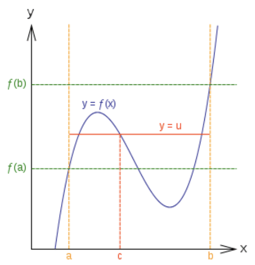
The Intermediate Value Theorem states that if a function is continuous on a closed interval and u is a value between f(a) and f(b) then there exists a c∈[a,b] such that f(c)=u.

CK-12 Foundation - http://commons.wikimedia.org/wiki/File:Intermediatevaluetheorem.svg - CC BY-SA
Simply stated, if a function is continuous between a low point and a high point, then it must be valued at each intermediate height in between the low and high points.
The converse of an if then statement is a new statement with the hypothesis of the original statement switched with the conclusion of the original statement. In other words, the converse is when the if part of the statement and the then part of the statement are swapped. In general, the converse of a statement is not true.
The converse of the Intermediate Value Theorem is: If there exists a value c∈[a,b] such that f(c)=u for every u between f(a) and f(b) then the function is continuous.
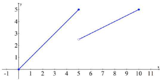
This statement is false. In order to show the statement is false, all you need is one counterexample where every intermediate value is hit and the function is discontinuous.A counterexample to an if then statement is when the hypothesis (the if part of the sentence) is true, but the conclusion (the then part of the statement) is not true.

CK-12 Foundation - CC BY-SA
This function is discontinuous on the interval [0,10] but every intermediate value between the first height at (0,0) and the height of the last point (10,5) is hit.
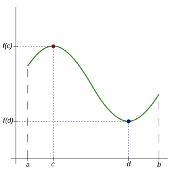
The Extreme Value Theorem states that in every interval [a,b] where a function is continuous there is at least one maximum and one minimum. In other words, it must have at least two extreme values.

CK-12 Foundation - http://commons.wikimedia.org/wiki/File:Extreme_Value_Theorem.svg;https://commons.wikimedia.org/wiki/File:CentralParkFromAboveCropped.jpg - CC BY-SA
The converse of the Extreme Value Theorem is: If there is at least one maximum and one minimum in the closed interval [a,b] then the function is continuous on [a,b].
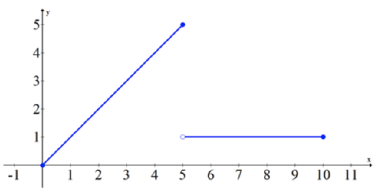
This statement is false. In order to show the statement is false, all you need is one counterexample. The goal is to find a function on a closed interval [a,b] that has at least one maximum and one minimum and is also discontinuous.

CK-12 Foundation - CC BY-SA
On the interval [0,10], the function attains a maximum at (5,5) and a minimum at (0,0) but is still discontinuous.
Examples
Example 1
Earlier, you were asked to apply the Intermediate and Extreme Value Theorems to a function is continuous on the interval x∈[1,4]. You can conclude by the Intermediate Value Theorem that there exists a c∈[1,4] such that f(c)=u for every u between f(1) and f(4). You can also conclude that on this interval the function has both a maximum and a minimum value by the Extreme Value Theorem.
Example 2
Use the Intermediate Value Theorem to show that the function f(x)=(x+1)3−4 has a zero on the interval [0,3].
First note that the function is a cubic and is therefore continuous everywhere.
- f(0)=(0+1)3−4=13−4=−3
- f(3)=(3+1)3−4=43−4=60
By the Intermediate Value Theorem, there must exist a c∈[0,3] such that f(c)=0 since 0 is between -3 and 60.
Example 3
Use the Intermediate Value Theorem to show that the following equation has at least one real solution.
x8=2x
First rewrite the equation: x8−2x=0
Then describe it as a continuous function: f(x)=x8−2x
This function is continuous because it is the difference of two continuous functions.
- f(0)=08−20=0−1=−1
- f(2)=28−22=256−4=252
By the Intermediate Value Theorem, there must exist a c such that f(c)=0 because −1<0<252. The number c is one solution to the initial equation.
Example 4
Show that there is at least one solution to the following equation.
sinx=x+2
Write the equation as a continuous function: f(x)=sinx−x−2
The function is continuous because it is the sum and difference of continuous functions.
- f(0)=sin0−0−2=−2
- f(−π)=sin(−π)+π−2=0+π−2>0
By the Intermediate Value Theorem, there must exist a c such that f(c)=0 because −2<0<π−2. The number c is one solution to the initial equation.
Example 5
When are you not allowed to use the Intermediate Value Theorem?
The Intermediate Value Theorem should not be applied when the function is not continuous over the interval.
Review
Use the Intermediate Value Theorem to show that each equation has at least one real solution.
1. cosx=−x
2. ln(x)=e−x+1
3. 2x3−5x2=10x−5
4. x3+1=x
5. x2=cosx
6. x5=2x3+2
7. 3x2+4x−11=0
8. 5x4=6x2+1
9. 7x3−18x2−4x+1=0
10. Show that f(x)=2x−3/2x−5 has a real root on the interval [1,2].
11. Show that f(x)=3x+1/2x+4 has a real root on the interval [−1,0].
12. True or false: A function has a maximum and a minimum in the closed interval [a,b]; therefore, the function is continuous.
13. True or false: A function is continuous over the interval [a,b]; therefore, the function has a maximum and a minimum in the closed interval.
14. True or false: If a function is continuous over the interval [a,b], then it is possible for the function to have more than one relative maximum in the interval [a,b].
15. What do the Intermediate Value and Extreme Value Theorems have to do with continuity?
Vocabulary
| Term | Definition |
|---|---|
| continuity | Continuity for a point exists when the left and right sided limits match the function evaluated at that point. For a function to be continuous, the function must be continuous at every single point in an unbroken domain. |
| Continuous | Continuity for a point exists when the left and right sided limits match the function evaluated at that point. For a function to be continuous, the function must be continuous at every single point in an unbroken domain. |
| converse | If a conditional statement is p→q (if p, then q), then the converse is q→p (if q, then p. Note that the converse of a statement is not true just because the original statement is true. |
| counterexample | A counterexample is an example that disproves a conjecture. |
| extreme value theorem | The extreme value theorem states that in every interval [a,b] where a function is continuous there is at least one maximum and one minimum. In other words, it must have at least two extreme values. |
| intermediate value theorem | The intermediate value theorem states that if f(x) is continuous on some interval [a,b] and n is between f(a) and f(b), then there is some c∈[a,b] such that f(c)=n. |
Additional Resources
PLIX: Play, Learn, Interact, eXplore - Function Exploration
Video: Descartes' Rule of Signs - Example 1
Practice: Intermediate Value Theorem, Existence of Solutions
Real World: Ups and Downs

