3.4: Find Imaginary Solutions

Louis calculates that the area of a rectangle is represented by the equation 3x⁴ + 7x² = 2. Did Louis calculate it right? Explain based on the degree and zeros of the function.

---

Imaginary Solutions

Remember, imaginary solutions always come in pairs. To find the imaginary solutions to a function, use the Quadratic Formula.

Let's solve f(x)=3x⁴−x²−14.

First, this quartic function can be factored just like a quadratic equation.

g(x)=x⁴+21x²+90

Now, because neither factor can be factored further and there is no x−term, we can set each equal to zero and solve.

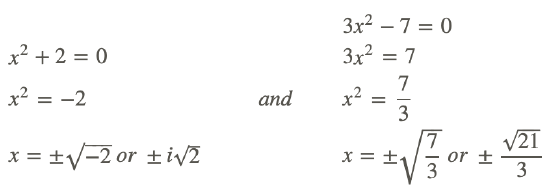
Including the imaginary solutions, there are four, which is what we would expect because the degree of this function is four.

Now, let's find all the solutions of the function g(x)=x⁴+21x²+90.

When graphed, this function does not touch the x−axis. Therefore, all the solutions are imaginary. To solve, this function can be factored like a quadratic equation. The factors of 90 that add up to 21 are 6 and 15.

g(x)0=x⁴+21x²+9

0=(x²+6)(x²+15)

Now, set each factor equal to zero and solve.

Finally, let's find the function that has the solution 3, -2, and 4+i.

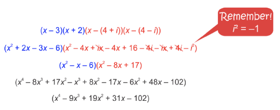
Notice that one of the given solutions involves an imaginary number. Imaginary and complex solutions always come in pairs, so 4−i is also a factor. The two factors are complex conjugates. Translate each solution into a factor and multiply them all together.

Bahman Kalantari - https://commons.wikimedia.org/wiki/File%3ANonfractal_polynomiograph.png

Any multiple of this function would also have these roots. For example, 2x4−18x3+38x2+62x−204 would have these roots as well.

---

Examples

Example 1

Earlier, you were asked to determine if Louis calculated his work correctly.

First we need to change the equation to standard form. Then we can factor it.

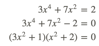
Solving for x we get

All of the solutions are imaginary and the area of a rectangle must have real solutions. Therefore Louis did not calculate correctly.

Example 2

Find all the solutions to the following function: f(x)=25x3−120x2+81x−4.

First, graph the function.

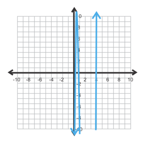
Using the Rational Root Theorem, the possible realistic zeros could be ¹/₂₅, 1, or 4. Let’s try these three possibilities using synthetic division.

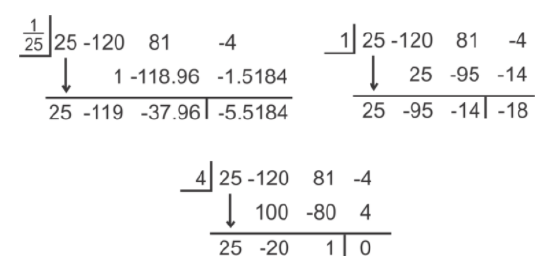
Of these three possibilities, only 4 is a zero. The leftover polynomial, 25x²−20x+1 is not factorable, so we need to use the Quadratic Formula to find the last two zeros.

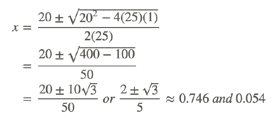
Helpful Hint: Always find the decimal values of each zero to make sure they match up with the graph.

Example 3

Find all the solutions to the following function: f(x)=4x⁴+35x²−9.

f(x)=4x⁴+35x²−9 is factorable. ac=−36.

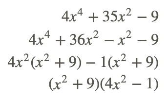
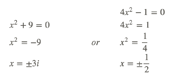
Setting each factor equal to zero, we have:

Example 4

Find the equation of a function with roots 4, 2^0.5 and 1−i.

Recall that irrational and imaginary roots come in pairs. Therefore, all the roots are 4, 2^0.5,−2^0.5,1+i,1−i. Multiply all 5 roots together.

---

Review

Find all solutions to the following functions. Use any method.

1. f(x)=x⁴+x³−12x²−10x+20
2. f(x)=4x³−20x²−3x+15
3. f(x)=2x⁴−7x²−30
4. f(x)=x³+5x²+12x+18
5. f(x)=4x⁴+4x³−22x²−8x+40
6. f(x)=3x⁴+4x²−15
7. f(x)=2x³−6x²+9x−27
8. f(x)=6x⁴−7x³−280x²−419x+280
9. f(x)=9x⁴+6x³−28x²+2x+11
10. f(x)=2x⁵−19x⁴+30x³+97x²−20x+150

Find a function with the following roots.

11. 4,i
12. −3,−2i
13. 5^0.5,−1+i
14. 2,13,4−2^0.5
15. Writing: Write down the steps you use to find all the zeros of a polynomial function.
16. Writing: Why do imaginary and irrational roots always come in pairs?
17. Challenge: Find all the solutions to f(x)=x5+x3+8x2+8.

---

Answers for Review Problems

To see the Review answers, open this PDF file and look for section 6.12.

---

Vocabulary

Term	Definition
Complex Conjugate	Complex conjugates are pairs of complex binomials. The complex conjugate of a+bi is a−bi. When complex conjugates are multiplied, the result is a single real number.
complex number	A complex number is the sum of a real number and an imaginary number, written in the form a+bi.
conjugate pairs theorem	The conjugate pairs theorem states that if f(z) is a polynomial of degree n, with n≠0 and with real coefficients, and if f(z0)=0, where z0=a+bi, then f(z∗0)=0. Where z∗0 is the complex conjugate of z0.
fundamental theorem of algebra	The fundamental theorem of algebra states that if f(x) is a polynomial of degree n≥1, then f(x) has at least one zero in the complex number domain. In other words, there is at least one complex number c such that f(c)=0. The theorem can also be stated as follows: an nth degree polynomial with real or complex coefficients has, with multiplicity, exactly n complex roots.
Imaginary Number	An imaginary number is a number that can be written as the product of a real number and i.
Imaginary Numbers	An imaginary number is a number that can be written as the product of a real number and i.
Polynomial	A polynomial is an expression with at least one algebraic term, but which does not indicate division by a variable or contain variables with fractional exponents.
Roots	The roots of a function are the values of x that make y equal to zero.
Zero	The zeros of a function f(x) are the values of x that cause f(x) to be equal to zero.
Zeroes	The zeroes of a function f(x) are the values of x that cause f(x) to be equal to zero.

---

Additional Resources

PLIX: Play, Learn, Interact, eXplore - Imaginary Zeros

Video: Fundamental Theorem of Algebra - Overview

Practice: Find Imaginary Solutions