3.1: Continuity of a Function
- Page ID
- 1196
\( \newcommand{\vecs}[1]{\overset { \scriptstyle \rightharpoonup} {\mathbf{#1}} } \)
\( \newcommand{\vecd}[1]{\overset{-\!-\!\rightharpoonup}{\vphantom{a}\smash {#1}}} \)
\( \newcommand{\dsum}{\displaystyle\sum\limits} \)
\( \newcommand{\dint}{\displaystyle\int\limits} \)
\( \newcommand{\dlim}{\displaystyle\lim\limits} \)
\( \newcommand{\id}{\mathrm{id}}\) \( \newcommand{\Span}{\mathrm{span}}\)
( \newcommand{\kernel}{\mathrm{null}\,}\) \( \newcommand{\range}{\mathrm{range}\,}\)
\( \newcommand{\RealPart}{\mathrm{Re}}\) \( \newcommand{\ImaginaryPart}{\mathrm{Im}}\)
\( \newcommand{\Argument}{\mathrm{Arg}}\) \( \newcommand{\norm}[1]{\| #1 \|}\)
\( \newcommand{\inner}[2]{\langle #1, #2 \rangle}\)
\( \newcommand{\Span}{\mathrm{span}}\)
\( \newcommand{\id}{\mathrm{id}}\)
\( \newcommand{\Span}{\mathrm{span}}\)
\( \newcommand{\kernel}{\mathrm{null}\,}\)
\( \newcommand{\range}{\mathrm{range}\,}\)
\( \newcommand{\RealPart}{\mathrm{Re}}\)
\( \newcommand{\ImaginaryPart}{\mathrm{Im}}\)
\( \newcommand{\Argument}{\mathrm{Arg}}\)
\( \newcommand{\norm}[1]{\| #1 \|}\)
\( \newcommand{\inner}[2]{\langle #1, #2 \rangle}\)
\( \newcommand{\Span}{\mathrm{span}}\) \( \newcommand{\AA}{\unicode[.8,0]{x212B}}\)
\( \newcommand{\vectorA}[1]{\vec{#1}} % arrow\)
\( \newcommand{\vectorAt}[1]{\vec{\text{#1}}} % arrow\)
\( \newcommand{\vectorB}[1]{\overset { \scriptstyle \rightharpoonup} {\mathbf{#1}} } \)
\( \newcommand{\vectorC}[1]{\textbf{#1}} \)
\( \newcommand{\vectorD}[1]{\overrightarrow{#1}} \)
\( \newcommand{\vectorDt}[1]{\overrightarrow{\text{#1}}} \)
\( \newcommand{\vectE}[1]{\overset{-\!-\!\rightharpoonup}{\vphantom{a}\smash{\mathbf {#1}}}} \)
\( \newcommand{\vecs}[1]{\overset { \scriptstyle \rightharpoonup} {\mathbf{#1}} } \)
\(\newcommand{\longvect}{\overrightarrow}\)
\( \newcommand{\vecd}[1]{\overset{-\!-\!\rightharpoonup}{\vphantom{a}\smash {#1}}} \)
\(\newcommand{\avec}{\mathbf a}\) \(\newcommand{\bvec}{\mathbf b}\) \(\newcommand{\cvec}{\mathbf c}\) \(\newcommand{\dvec}{\mathbf d}\) \(\newcommand{\dtil}{\widetilde{\mathbf d}}\) \(\newcommand{\evec}{\mathbf e}\) \(\newcommand{\fvec}{\mathbf f}\) \(\newcommand{\nvec}{\mathbf n}\) \(\newcommand{\pvec}{\mathbf p}\) \(\newcommand{\qvec}{\mathbf q}\) \(\newcommand{\svec}{\mathbf s}\) \(\newcommand{\tvec}{\mathbf t}\) \(\newcommand{\uvec}{\mathbf u}\) \(\newcommand{\vvec}{\mathbf v}\) \(\newcommand{\wvec}{\mathbf w}\) \(\newcommand{\xvec}{\mathbf x}\) \(\newcommand{\yvec}{\mathbf y}\) \(\newcommand{\zvec}{\mathbf z}\) \(\newcommand{\rvec}{\mathbf r}\) \(\newcommand{\mvec}{\mathbf m}\) \(\newcommand{\zerovec}{\mathbf 0}\) \(\newcommand{\onevec}{\mathbf 1}\) \(\newcommand{\real}{\mathbb R}\) \(\newcommand{\twovec}[2]{\left[\begin{array}{r}#1 \\ #2 \end{array}\right]}\) \(\newcommand{\ctwovec}[2]{\left[\begin{array}{c}#1 \\ #2 \end{array}\right]}\) \(\newcommand{\threevec}[3]{\left[\begin{array}{r}#1 \\ #2 \\ #3 \end{array}\right]}\) \(\newcommand{\cthreevec}[3]{\left[\begin{array}{c}#1 \\ #2 \\ #3 \end{array}\right]}\) \(\newcommand{\fourvec}[4]{\left[\begin{array}{r}#1 \\ #2 \\ #3 \\ #4 \end{array}\right]}\) \(\newcommand{\cfourvec}[4]{\left[\begin{array}{c}#1 \\ #2 \\ #3 \\ #4 \end{array}\right]}\) \(\newcommand{\fivevec}[5]{\left[\begin{array}{r}#1 \\ #2 \\ #3 \\ #4 \\ #5 \\ \end{array}\right]}\) \(\newcommand{\cfivevec}[5]{\left[\begin{array}{c}#1 \\ #2 \\ #3 \\ #4 \\ #5 \\ \end{array}\right]}\) \(\newcommand{\mattwo}[4]{\left[\begin{array}{rr}#1 \amp #2 \\ #3 \amp #4 \\ \end{array}\right]}\) \(\newcommand{\laspan}[1]{\text{Span}\{#1\}}\) \(\newcommand{\bcal}{\cal B}\) \(\newcommand{\ccal}{\cal C}\) \(\newcommand{\scal}{\cal S}\) \(\newcommand{\wcal}{\cal W}\) \(\newcommand{\ecal}{\cal E}\) \(\newcommand{\coords}[2]{\left\{#1\right\}_{#2}}\) \(\newcommand{\gray}[1]{\color{gray}{#1}}\) \(\newcommand{\lgray}[1]{\color{lightgray}{#1}}\) \(\newcommand{\rank}{\operatorname{rank}}\) \(\newcommand{\row}{\text{Row}}\) \(\newcommand{\col}{\text{Col}}\) \(\renewcommand{\row}{\text{Row}}\) \(\newcommand{\nul}{\text{Nul}}\) \(\newcommand{\var}{\text{Var}}\) \(\newcommand{\corr}{\text{corr}}\) \(\newcommand{\len}[1]{\left|#1\right|}\) \(\newcommand{\bbar}{\overline{\bvec}}\) \(\newcommand{\bhat}{\widehat{\bvec}}\) \(\newcommand{\bperp}{\bvec^\perp}\) \(\newcommand{\xhat}{\widehat{\xvec}}\) \(\newcommand{\vhat}{\widehat{\vvec}}\) \(\newcommand{\uhat}{\widehat{\uvec}}\) \(\newcommand{\what}{\widehat{\wvec}}\) \(\newcommand{\Sighat}{\widehat{\Sigma}}\) \(\newcommand{\lt}{<}\) \(\newcommand{\gt}{>}\) \(\newcommand{\amp}{&}\) \(\definecolor{fillinmathshade}{gray}{0.9}\)The continuity of a function is related to the conceptual notion of a function not having any breaks or sudden jumps as the independent variable takes on all values over some interval. There are no range gaps, or sudden jumps over the domain of interest. With this in mind, see if you can determine which of the following could be considered to represent a continuous function:
- daily outdoor temperature variation
- weight of a cart as 10 lb bags of sand are loaded on it
- the rise and fall of the level of a reservoir of water
- the amount of money collected at a movie theater for a specific showing.
Continuity
Continuity of a function is conceptually the characteristic of a function curve that has the values of the range “flow” continuously without interruption over some interval, as if never having to lift pencil from paper while drawing the curve. This intuitive notion needs to be formalized mathematically.
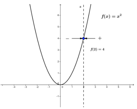
Consider the graph of the function f(x)=x2. The function is defined for any real value of the independent variable.
CK-12 Foundation - CC BY-NC-SA
For example, for x=2 the function has the value f(2)=4. Notice that as x approaches the value 2 from either the left or the right, the value of the function approaches 4, i.e.
\[\lim _{x \rightarrow 2} f(x)=f(2)=4\]
Conceptually, applying the left and right one-sided limits as x approached 2, resulted in the same value, the value of the function at x=2.
The above results illustrate key properties of a continuous function. They are formalized in the following definition that provides a test for determining when we have a continuous function.
The function f(x) is continuous at x=a if the following conditions all hold:
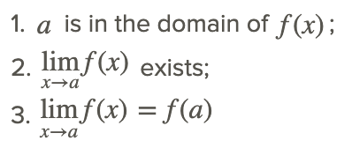
Note that it is possible to have functions where two of these conditions are satisfied but the third is not. When a function is not continuous at x=a, then it is discontinuous at a, and a is a point of discontinuity.
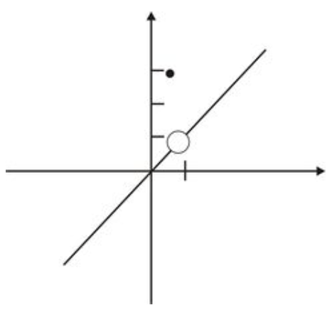
Consider the piece-wise function
\[f(x)=\left\{\begin{array}{l}
x, \text { if } x \neq 1 \\
3, \text { if } x=1
\end{array}\right.\]
with the graph shown below.
CK-12 Foundation - CC BY-NC-SA
In this example, we have
\[\lim _{x \rightarrow 1} f(x)\]
exists! The value x=1 is in the domain of f(x), but
\[\lim _{x \rightarrow 1} f(x) \neq f(1)\]
Therefore the function is not continuous at x=1.
This is an example of a removable discontinuity, i.e., a discontinuity at which the limit of the function exists but does not equal the value of the function at that point.
Consider the following function:
\[f(x)=\frac{(x+1)}{\left(x^{2}-1\right)}\]
Are there any discontinuities?
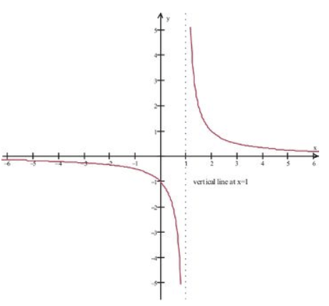
We know from our study of domains that in order for the function to be defined, we must have x≠−1,1. Yet when we generate the graph of the function (using the standard viewing window), we get the following picture that appears to be defined at x=−1:
CK-12 Foundation - CC BY-NC-SA
The apparent contradiction is due to the fact that our original function had x+1 as a common factor in the numerator and denominator, which cancelled out and gave us a picture that appears to be the graph of
\[f(x)=\frac{1}{(x-1)}\]
But what we actually have is the original function,
\[f(x)=\frac{(x+1)}{\left(x^{2}-1\right)}\]
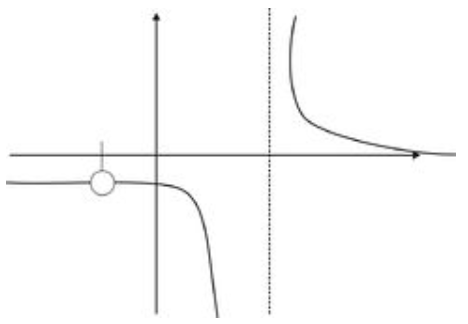
that we know is not defined at x=−1. At x=−1, we have a hole in the graph, or a discontinuity of the function at x=−1. That is, the function is defined for all other x-values close to x=−1.
In addition, at x=1 the function values go to ±∞ depending on which side of x=1 is used. The right and left one-sided limits will not be the same, and the function is discontinuous at x=1. The discontinuity at x=1 is called an infinite discontinuity and is associated with the vertical asymptote x=1.
Loosely speaking, if we were to hand-draw the graph, we would need to take our pencil off the page when we got to this hole, leaving a gap in the graph as indicated:
CK-12 Foundation - CC BY-NC-SA
Examples
Example 1
Earlier, you were asked which of the following could be considered to represent a continuous function:
- daily outdoor temperature variation
- weight of a cart as 10 lb bags of sand are loaded
- the rise and fall of the level of water in a reservoir
- the amount of money collected at a movie theater for a specific showing
The daily outdoor temperature variation could be considered a continuous function of time as because all temperature values occur in the range of variation.
The weight of a cart as 10 lb bags of sand are loaded would not be considered a continuous function of the number of bags because only integer numbers of bags are possible and the total weight changes in 10 lb increments, so there are gaps.
The rise and fall of the level of water in a reservoir could be considered continuous function of time because all levels occur in the range of variation.
The amount of money collected at a movie theater for a specific showing would not be considered a continuous function since the number of people buying and the price per ticket are integers so that only certain total dollar amounts are possible.
Example 2
Find a value of k which makes the following function continuous:

If f(x) is to be considered continuous everywhere, it must be continuous at x=3. This means that:

Then

With the above result, we have

Therefore, the function

is continuous at x=3.
Example 3
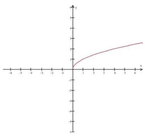
Let’s recall our basic square root function, f(x)=x0.5, shown below. Is it continuous at x=0?
CK-12 Foundation - CC BY-NC-SA
Since the domain of f(x)=x0.5 is x≥0, we see that
\[\lim _{x \rightarrow 0} \sqrt{x}\]
does not exist. Specifically, we cannot find open intervals around \(x=0\) that satisfy the limit definition. Therefore, the function is not continuous at \(x=0\). However we do note that as we approach x=0 from the right-hand side, we see the successive values tending towards \(x=0\).
Review
Vocabulary
| Term | Definition |
|---|---|
| Continuous | Continuity for a point exists when the left and right sided limits match the function evaluated at that point. For a function to be continuous, the function must be continuous at every single point in an unbroken domain. |
| Continuous Function | A continuous function is a function without breaks or gaps. It contains an infinite, uncountable number of values. |
| discontinuities | The points of discontinuity for a function are the input values of the function where the function is discontinuous. |
| discontinuous | A function is discontinuous if the function exhibits breaks or holes when graphed. |
| discontinuous at a point | A function is discontinuous at a point a if the function is not defined at x=a. |
| Infinite discontinuities | Infinite discontinuities occur when a function has a vertical asymptote on one or both sides. This will happen when a factor in the denominator of the function is zero. |
| Infinite discontinuity | Infinite discontinuities occur when a function has a vertical asymptote on one or both sides. This will happen when a factor in the denominator of the function is zero. |
| points of discontinuity | The points of discontinuity for a function are the input values of the function where the function is discontinuous. |
| Removable discontinuities | Removable discontinuities are also known as holes. They occur when factors can be algebraically canceled from rational functions. |
| Removable discontinuity | Removable discontinuities are also known as holes. They occur when factors can be algebraically canceled from rational functions. |
Additional Resources
PLIX: Play, Learn, Interact, eXplore - Continuity
Video: Continuity Using Limits
Practice: Continuity of a Function
Real World: Mitochondrial DNA

