1.8: 1.8 Zeroes and Intercepts of Functions
- Page ID
- 11453
\( \newcommand{\vecs}[1]{\overset { \scriptstyle \rightharpoonup} {\mathbf{#1}} } \)
\( \newcommand{\vecd}[1]{\overset{-\!-\!\rightharpoonup}{\vphantom{a}\smash {#1}}} \)
\( \newcommand{\dsum}{\displaystyle\sum\limits} \)
\( \newcommand{\dint}{\displaystyle\int\limits} \)
\( \newcommand{\dlim}{\displaystyle\lim\limits} \)
\( \newcommand{\id}{\mathrm{id}}\) \( \newcommand{\Span}{\mathrm{span}}\)
( \newcommand{\kernel}{\mathrm{null}\,}\) \( \newcommand{\range}{\mathrm{range}\,}\)
\( \newcommand{\RealPart}{\mathrm{Re}}\) \( \newcommand{\ImaginaryPart}{\mathrm{Im}}\)
\( \newcommand{\Argument}{\mathrm{Arg}}\) \( \newcommand{\norm}[1]{\| #1 \|}\)
\( \newcommand{\inner}[2]{\langle #1, #2 \rangle}\)
\( \newcommand{\Span}{\mathrm{span}}\)
\( \newcommand{\id}{\mathrm{id}}\)
\( \newcommand{\Span}{\mathrm{span}}\)
\( \newcommand{\kernel}{\mathrm{null}\,}\)
\( \newcommand{\range}{\mathrm{range}\,}\)
\( \newcommand{\RealPart}{\mathrm{Re}}\)
\( \newcommand{\ImaginaryPart}{\mathrm{Im}}\)
\( \newcommand{\Argument}{\mathrm{Arg}}\)
\( \newcommand{\norm}[1]{\| #1 \|}\)
\( \newcommand{\inner}[2]{\langle #1, #2 \rangle}\)
\( \newcommand{\Span}{\mathrm{span}}\) \( \newcommand{\AA}{\unicode[.8,0]{x212B}}\)
\( \newcommand{\vectorA}[1]{\vec{#1}} % arrow\)
\( \newcommand{\vectorAt}[1]{\vec{\text{#1}}} % arrow\)
\( \newcommand{\vectorB}[1]{\overset { \scriptstyle \rightharpoonup} {\mathbf{#1}} } \)
\( \newcommand{\vectorC}[1]{\textbf{#1}} \)
\( \newcommand{\vectorD}[1]{\overrightarrow{#1}} \)
\( \newcommand{\vectorDt}[1]{\overrightarrow{\text{#1}}} \)
\( \newcommand{\vectE}[1]{\overset{-\!-\!\rightharpoonup}{\vphantom{a}\smash{\mathbf {#1}}}} \)
\( \newcommand{\vecs}[1]{\overset { \scriptstyle \rightharpoonup} {\mathbf{#1}} } \)
\(\newcommand{\longvect}{\overrightarrow}\)
\( \newcommand{\vecd}[1]{\overset{-\!-\!\rightharpoonup}{\vphantom{a}\smash {#1}}} \)
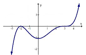
\(\newcommand{\avec}{\mathbf a}\) \(\newcommand{\bvec}{\mathbf b}\) \(\newcommand{\cvec}{\mathbf c}\) \(\newcommand{\dvec}{\mathbf d}\) \(\newcommand{\dtil}{\widetilde{\mathbf d}}\) \(\newcommand{\evec}{\mathbf e}\) \(\newcommand{\fvec}{\mathbf f}\) \(\newcommand{\nvec}{\mathbf n}\) \(\newcommand{\pvec}{\mathbf p}\) \(\newcommand{\qvec}{\mathbf q}\) \(\newcommand{\svec}{\mathbf s}\) \(\newcommand{\tvec}{\mathbf t}\) \(\newcommand{\uvec}{\mathbf u}\) \(\newcommand{\vvec}{\mathbf v}\) \(\newcommand{\wvec}{\mathbf w}\) \(\newcommand{\xvec}{\mathbf x}\) \(\newcommand{\yvec}{\mathbf y}\) \(\newcommand{\zvec}{\mathbf z}\) \(\newcommand{\rvec}{\mathbf r}\) \(\newcommand{\mvec}{\mathbf m}\) \(\newcommand{\zerovec}{\mathbf 0}\) \(\newcommand{\onevec}{\mathbf 1}\) \(\newcommand{\real}{\mathbb R}\) \(\newcommand{\twovec}[2]{\left[\begin{array}{r}#1 \\ #2 \end{array}\right]}\) \(\newcommand{\ctwovec}[2]{\left[\begin{array}{c}#1 \\ #2 \end{array}\right]}\) \(\newcommand{\threevec}[3]{\left[\begin{array}{r}#1 \\ #2 \\ #3 \end{array}\right]}\) \(\newcommand{\cthreevec}[3]{\left[\begin{array}{c}#1 \\ #2 \\ #3 \end{array}\right]}\) \(\newcommand{\fourvec}[4]{\left[\begin{array}{r}#1 \\ #2 \\ #3 \\ #4 \end{array}\right]}\) \(\newcommand{\cfourvec}[4]{\left[\begin{array}{c}#1 \\ #2 \\ #3 \\ #4 \end{array}\right]}\) \(\newcommand{\fivevec}[5]{\left[\begin{array}{r}#1 \\ #2 \\ #3 \\ #4 \\ #5 \\ \end{array}\right]}\) \(\newcommand{\cfivevec}[5]{\left[\begin{array}{c}#1 \\ #2 \\ #3 \\ #4 \\ #5 \\ \end{array}\right]}\) \(\newcommand{\mattwo}[4]{\left[\begin{array}{rr}#1 \amp #2 \\ #3 \amp #4 \\ \end{array}\right]}\) \(\newcommand{\laspan}[1]{\text{Span}\{#1\}}\) \(\newcommand{\bcal}{\cal B}\) \(\newcommand{\ccal}{\cal C}\) \(\newcommand{\scal}{\cal S}\) \(\newcommand{\wcal}{\cal W}\) \(\newcommand{\ecal}{\cal E}\) \(\newcommand{\coords}[2]{\left\{#1\right\}_{#2}}\) \(\newcommand{\gray}[1]{\color{gray}{#1}}\) \(\newcommand{\lgray}[1]{\color{lightgray}{#1}}\) \(\newcommand{\rank}{\operatorname{rank}}\) \(\newcommand{\row}{\text{Row}}\) \(\newcommand{\col}{\text{Col}}\) \(\renewcommand{\row}{\text{Row}}\) \(\newcommand{\nul}{\text{Nul}}\) \(\newcommand{\var}{\text{Var}}\) \(\newcommand{\corr}{\text{corr}}\) \(\newcommand{\len}[1]{\left|#1\right|}\) \(\newcommand{\bbar}{\overline{\bvec}}\) \(\newcommand{\bhat}{\widehat{\bvec}}\) \(\newcommand{\bperp}{\bvec^\perp}\) \(\newcommand{\xhat}{\widehat{\xvec}}\) \(\newcommand{\vhat}{\widehat{\vvec}}\) \(\newcommand{\uhat}{\widehat{\uvec}}\) \(\newcommand{\what}{\widehat{\wvec}}\) \(\newcommand{\Sighat}{\widehat{\Sigma}}\) \(\newcommand{\lt}{<}\) \(\newcommand{\gt}{>}\) \(\newcommand{\amp}{&}\) \(\definecolor{fillinmathshade}{gray}{0.9}\)An intercept in mathematics is where a function crosses the \(x\) or \(y\) axis. What are
the intercepts of this function?
X and Y Intercepts
The first type of intercept you may have learned is the \(y\) -intercept when you learned the slope intercept form of a line: \(y=m x+b\). A \(y\) -intercept is the unique point where a function crosses the \(y\) axis. It can be found algebraically by setting \(x=0\) and solving for \(y\).
\(x\) -intercepts are where functions cross the \(x\) axis and where the height of thefunction is zero. They are also called roots, solutions and zeroes of a function. They are found algebraically by setting \(y=0\) and solving for \(x\). Watch the videos below for practice:
Examples
Earlier, you were asked what the intercepts of the graph below are.
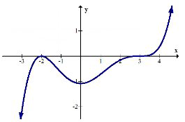
Graphically the function has zeroes at -2 and 3 with a \(y\) intercept at about \(-1.1 .\)
Note: In order for a function to pass the vertical line test, it must only have one \(y\) -intercept, but it may have multiple \(x\) -intercepts.
What are the zeroes and \(y\) -intercepts of the parabola \(y=x^{2}-2 x-3 ?\)
Using a graph:
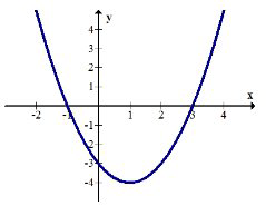
The zeroes are at (-1,0) and (3,0) . The \(y\) -intercept is at (0,-3) .
Using Algebra:
Substitute 0 for \(y\) to find zeroes.
\(0=x^{2}-2 x-3=(x-3)(x+1)\)
\(y=0, x=3,-1\)
Substitute 0 for \(x\) to find the \(y\) -intercept.
\(y=(0)^{2}-2(0)-3=-3\)
\(x=0, y=-3\)
Identify the zeroes and \(y\) -intercepts for the sine function.
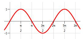
The \(y\) -intercept is (0,0) . There are four zeroes visible on this portion of the graph. One thing you know about the sine graph is that it is periodic and repeats forever in both directions. In order to capture every \(x\) -intercept, you must identify a pattern instead of trying to write out every single one.
The visible \(x\) -intercepts are \(0, \pi, 2 \pi, 3 \pi\). The pattern is that there is an \(x\) -intercept every multiple of \(\pi\) including negative multiples. In order to describe all of these values you should write:
The \(x\) -intercepts are \(\pm n \pi\) where \(n\) is an integer \(\{0,\pm 1,\pm 2, \ldots\}\).
Identify the intercepts and zeroes of the function: \(f(x)=\frac{1}{100}(x-3)^{3}(x+2)^{2}\)
To find the \(y\) -intercept, substitute o for \(x\) :
\(y=\frac{1}{100}(0-3)^{3}(0+2)^{2}=\frac{1}{100}(-27)(4)=-\frac{108}{100}=-1.08\)
To find the \(x\) -intercepts, substitute 0 for \(y\) :
\(0=\frac{1}{100}(x-3)^{3}(x+2)^{2}\)
\(x=3,-2\)
Thus the \(y\) -intercept is (0,-1.08) and the \(x\) -intercepts are (3,0) and (-2,0)
Determine the intercepts of the following function graphically.
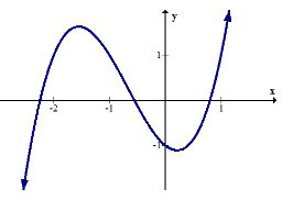
The \(y\) -intercept is approximately (0,-1) . The \(x\) -intercepts are approximately (-2.3,0), (-0.4,0) and \((0.7,0) .\) When finding values graphically, answers are always approximate. Exact answers need to be found analytically.
Review
1. Determine the zeroes and \(y\) -intercept of the following function using algebra:
\(f(x)=(x+1)^{3}(x-4)\)
2. Determine the roots and \(y\) -intercept of the following function using algebra or a graph:
3. Determine the intercepts of the following function graphically:
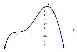
Find the intercepts for each of the following functions.
4. \(y=x^{2}\)
5. \(y=x^{3}\)
6. \(y=\ln (x)\)
7. \(y=\frac{1}{x}\)
8. \(y=e^{x}\)
9. \(y=\sqrt{x}\)
10. Are there any functions without a \(y\) -intercept? Explain.
11. Are there any functions without an \(x\) -intercept? Explain.
12. Explain why it makes sense that an \(x\) -intercept of a function is also called a
"zero" of the function.
Determine the intercepts of the following functions using algebra or a graph.
13. \(h(x)=x^{3}-6 x^{2}+3 x+10\)
14. \(j(x)=x^{2}-6 x-7\)
15. \(k(x)=4 x^{4}-20 x^{3}-3 x^{2}+14 x+5\)

