2.9.2: Applications of Box-and-Whisker Plots
- Page ID
- 5779
\( \newcommand{\vecs}[1]{\overset { \scriptstyle \rightharpoonup} {\mathbf{#1}} } \)
\( \newcommand{\vecd}[1]{\overset{-\!-\!\rightharpoonup}{\vphantom{a}\smash {#1}}} \)
\( \newcommand{\id}{\mathrm{id}}\) \( \newcommand{\Span}{\mathrm{span}}\)
( \newcommand{\kernel}{\mathrm{null}\,}\) \( \newcommand{\range}{\mathrm{range}\,}\)
\( \newcommand{\RealPart}{\mathrm{Re}}\) \( \newcommand{\ImaginaryPart}{\mathrm{Im}}\)
\( \newcommand{\Argument}{\mathrm{Arg}}\) \( \newcommand{\norm}[1]{\| #1 \|}\)
\( \newcommand{\inner}[2]{\langle #1, #2 \rangle}\)
\( \newcommand{\Span}{\mathrm{span}}\)
\( \newcommand{\id}{\mathrm{id}}\)
\( \newcommand{\Span}{\mathrm{span}}\)
\( \newcommand{\kernel}{\mathrm{null}\,}\)
\( \newcommand{\range}{\mathrm{range}\,}\)
\( \newcommand{\RealPart}{\mathrm{Re}}\)
\( \newcommand{\ImaginaryPart}{\mathrm{Im}}\)
\( \newcommand{\Argument}{\mathrm{Arg}}\)
\( \newcommand{\norm}[1]{\| #1 \|}\)
\( \newcommand{\inner}[2]{\langle #1, #2 \rangle}\)
\( \newcommand{\Span}{\mathrm{span}}\) \( \newcommand{\AA}{\unicode[.8,0]{x212B}}\)
\( \newcommand{\vectorA}[1]{\vec{#1}} % arrow\)
\( \newcommand{\vectorAt}[1]{\vec{\text{#1}}} % arrow\)
\( \newcommand{\vectorB}[1]{\overset { \scriptstyle \rightharpoonup} {\mathbf{#1}} } \)
\( \newcommand{\vectorC}[1]{\textbf{#1}} \)
\( \newcommand{\vectorD}[1]{\overrightarrow{#1}} \)
\( \newcommand{\vectorDt}[1]{\overrightarrow{\text{#1}}} \)
\( \newcommand{\vectE}[1]{\overset{-\!-\!\rightharpoonup}{\vphantom{a}\smash{\mathbf {#1}}}} \)
\( \newcommand{\vecs}[1]{\overset { \scriptstyle \rightharpoonup} {\mathbf{#1}} } \)
\( \newcommand{\vecd}[1]{\overset{-\!-\!\rightharpoonup}{\vphantom{a}\smash {#1}}} \)
\(\newcommand{\avec}{\mathbf a}\) \(\newcommand{\bvec}{\mathbf b}\) \(\newcommand{\cvec}{\mathbf c}\) \(\newcommand{\dvec}{\mathbf d}\) \(\newcommand{\dtil}{\widetilde{\mathbf d}}\) \(\newcommand{\evec}{\mathbf e}\) \(\newcommand{\fvec}{\mathbf f}\) \(\newcommand{\nvec}{\mathbf n}\) \(\newcommand{\pvec}{\mathbf p}\) \(\newcommand{\qvec}{\mathbf q}\) \(\newcommand{\svec}{\mathbf s}\) \(\newcommand{\tvec}{\mathbf t}\) \(\newcommand{\uvec}{\mathbf u}\) \(\newcommand{\vvec}{\mathbf v}\) \(\newcommand{\wvec}{\mathbf w}\) \(\newcommand{\xvec}{\mathbf x}\) \(\newcommand{\yvec}{\mathbf y}\) \(\newcommand{\zvec}{\mathbf z}\) \(\newcommand{\rvec}{\mathbf r}\) \(\newcommand{\mvec}{\mathbf m}\) \(\newcommand{\zerovec}{\mathbf 0}\) \(\newcommand{\onevec}{\mathbf 1}\) \(\newcommand{\real}{\mathbb R}\) \(\newcommand{\twovec}[2]{\left[\begin{array}{r}#1 \\ #2 \end{array}\right]}\) \(\newcommand{\ctwovec}[2]{\left[\begin{array}{c}#1 \\ #2 \end{array}\right]}\) \(\newcommand{\threevec}[3]{\left[\begin{array}{r}#1 \\ #2 \\ #3 \end{array}\right]}\) \(\newcommand{\cthreevec}[3]{\left[\begin{array}{c}#1 \\ #2 \\ #3 \end{array}\right]}\) \(\newcommand{\fourvec}[4]{\left[\begin{array}{r}#1 \\ #2 \\ #3 \\ #4 \end{array}\right]}\) \(\newcommand{\cfourvec}[4]{\left[\begin{array}{c}#1 \\ #2 \\ #3 \\ #4 \end{array}\right]}\) \(\newcommand{\fivevec}[5]{\left[\begin{array}{r}#1 \\ #2 \\ #3 \\ #4 \\ #5 \\ \end{array}\right]}\) \(\newcommand{\cfivevec}[5]{\left[\begin{array}{c}#1 \\ #2 \\ #3 \\ #4 \\ #5 \\ \end{array}\right]}\) \(\newcommand{\mattwo}[4]{\left[\begin{array}{rr}#1 \amp #2 \\ #3 \amp #4 \\ \end{array}\right]}\) \(\newcommand{\laspan}[1]{\text{Span}\{#1\}}\) \(\newcommand{\bcal}{\cal B}\) \(\newcommand{\ccal}{\cal C}\) \(\newcommand{\scal}{\cal S}\) \(\newcommand{\wcal}{\cal W}\) \(\newcommand{\ecal}{\cal E}\) \(\newcommand{\coords}[2]{\left\{#1\right\}_{#2}}\) \(\newcommand{\gray}[1]{\color{gray}{#1}}\) \(\newcommand{\lgray}[1]{\color{lightgray}{#1}}\) \(\newcommand{\rank}{\operatorname{rank}}\) \(\newcommand{\row}{\text{Row}}\) \(\newcommand{\col}{\text{Col}}\) \(\renewcommand{\row}{\text{Row}}\) \(\newcommand{\nul}{\text{Nul}}\) \(\newcommand{\var}{\text{Var}}\) \(\newcommand{\corr}{\text{corr}}\) \(\newcommand{\len}[1]{\left|#1\right|}\) \(\newcommand{\bbar}{\overline{\bvec}}\) \(\newcommand{\bhat}{\widehat{\bvec}}\) \(\newcommand{\bperp}{\bvec^\perp}\) \(\newcommand{\xhat}{\widehat{\xvec}}\) \(\newcommand{\vhat}{\widehat{\vvec}}\) \(\newcommand{\uhat}{\widehat{\uvec}}\) \(\newcommand{\what}{\widehat{\wvec}}\) \(\newcommand{\Sighat}{\widehat{\Sigma}}\) \(\newcommand{\lt}{<}\) \(\newcommand{\gt}{>}\) \(\newcommand{\amp}{&}\) \(\definecolor{fillinmathshade}{gray}{0.9}\)Using Box-and-Whisker Plots to Understand Data

A truck is carrying books packaged in boxes. The number of books in each box is recorded as shown.
| 15 | 1 | 20 | 7 | 15 | 8 | 3 | 20 |
| 8 | 16 | 3 | 4 | 13 | 17 | 20 | 9 |
| 6 | 16 | 22 | 12 | 6 | 19 | 7 | 9 |
| 10 | 15 | 9 | 18 | 19 | 15 | 14 | 15 |
| 2 | 28 | 10 | 17 | 7 | 10 | 8 | 8 |
a. Construct a box and whisker plot to represent the data.
b. What do you think is a “typical” number of books in a box? Justify your answer.
c. Are their outliers? Explain.
In this concept, you will learn to use box-and-whisker plots to understand data.
Box and Whisker Plots
At times it is useful to get a general idea of how data clusters together. Box-and-whisker plots display the distribution of data items along a number line. A box-and-whisker plot is created by determining five points. The data are divided into four equal parts, separated by points called quartiles. The smallest data point (the extreme minimum) and the largest data point (the extreme maximum) are also displayed on the graph.
First, arrange the data in order from smallest to largest. Then, create a number line that shows the range of the data using equal intervals. Use the median as the middle point on the box-and-whisker plot and to split the data in half. The median of each half, the quartile, is then calculated. These separate the data into quarters. Finally, use the smallest data value and the largest data value as the endpoints or extremes. Boxes are then drawn between the quartiles and whiskers are drawn to the extremes.
A box-and-whisker plot that is already constructed can quickly supply statistical measures by looking at the five points. The first and last points give the extremes of the data. The third or middle point gives the median of all the data. The second and fourth points, between the median and the extremes, give the quartiles.
The interquartile range is the range between the first quartile and the third quartile. This shows where the middle half of the data is located. It can be calculated by subtracting the first quartile from the third quartile.
Finally, the outliers, data items that are far away from the general trend, can be located as extremes that cause the whiskers to be exceptionally long. Data does not always have outliers. If there isn’t a single point that is exceptionally far from other points, then an outlier doesn’t exist.
Let’s look at an example.
Use the given box-and-whisker plot to identify: a) the extremes, b) the median, c) the quartiles, d) the interquartile range, and e) the outliers (if any).
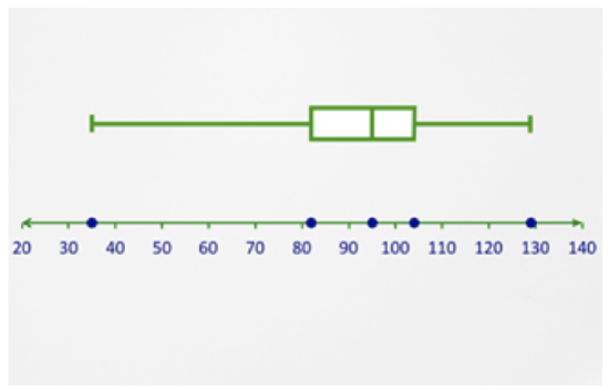
a. The extremes in this data set are approximately 35 and 129.
b. The median is approximately 95.
c. The first quartile is approximately 82 and the third quartile approximately 104.
d. The interquartile range, then, is 104 – 82 or 22.
e. Finally, the extreme minimum, 35, appears to be an outlier as the left whisker is very long compared to the rest of the plot.
Outliers are points that are unusually large or small compared to the rest of the data. When you discuss measures of central tendency like mean, median, and mode, you must also remember that in the real world there are many exceptions. Sometimes when you consider data, you might choose to remove the outliers in order to draw better conclusions based on the data.
Take a look at how removing an outlier can affect the interpretation of the data.
Sandra runs on her school’s track team. They recently ran a 100 meter dash at a track meet and recorded official times. These are the results in seconds:
11.7, 10.8, 11.1, 10.9, 11.7, 11.6, 12.0, 19.6, 12.2, 11.6, 11.5, 11.6, 11.0, 12.0, 11.6, 11.5, 11.7, 11.3, 12.3, 10.1.
Sandra’s time was 11.1 and she wants to know how she compares to the rest of her team. She will use a box-and-whisker plot to help figure this out.
First, she places the data in order.
10.1, 10.8, 10.9, 11.0, 11.1, 11.3, 11.5, 11.5, 11.6, 11.6, 11.6, 11.6, 11.7, 11.7, 11.7, 12.0, 12.0, 12.2, 12.3, 19.6
Next, she draws a number line that includes the extremes.
The extreme maximum is 19.6 and the extreme minimum is 10.1.
The number line is drawn from 9 to 21.
Then, she finds the median and places this number on the number line.
The median is the middle data value. There are 20 data points. The 10th and 11th data values are both 11.6. The median is 11.6.
Then, she finds the first and third quartiles and places these numbers on the number line.
She finds the median of the two groups above and below the median of the data set.
Group 1:
10.1, 10.8, 10.9, 11.0, 11.1, 11.3, 11.5, 11.5, 11.6, 11.6
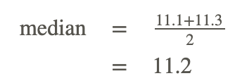
Group 2:
11.6, 11.6, 11.7, 11.7, 11.7, 12.0, 12.0, 12.2, 12.3, 19.6
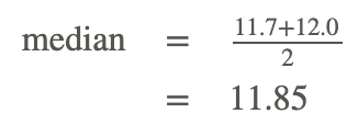
Then, she draws boxes between the quartiles and the median. She places the extremes, 10.1 and 19.6, on the numbers with points. She finally draws whiskers from the quartiles to the extremes.
Her diagram is below.
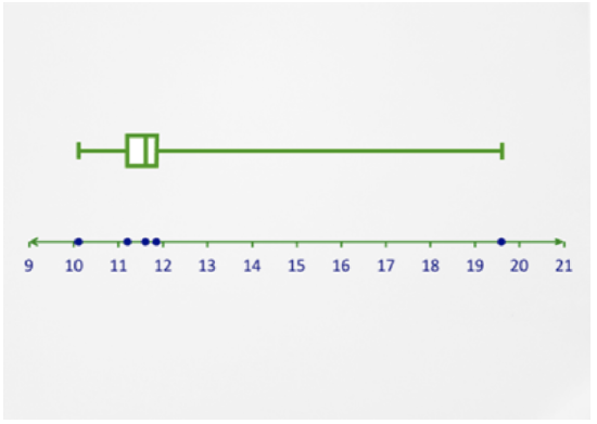
When Sandra analyzes the box-and-whisker plot, she finds that her time, 11.1 seconds, is barely less than the first quartile. She knows that her friend, Teresa, is fast with a time of 10.1. Another teammate, Lisa, had fallen during the race but got up and continued to the finish line. Her time was 19.6.
Sandra believes that neither Teresa nor Lisa’s scores are useful in gauging her speed. She decides to look at the same data but remove those two outliers.
Here’s her new data:
10.8, 10.9, 11.0, 11.1, 11.3, 11.5, 11.5, 11.6, 11.6, 11.6, 11.6, 11.7, 11.7, 11.7, 12.0, 12.0, 12.2, 12.3
She recalculates her statistical measures and creates a new box-and-whisker plot:
Extremes: 10.8 and 12.3
Median: 11.6
First and third quartiles: 11.3 and 11.7
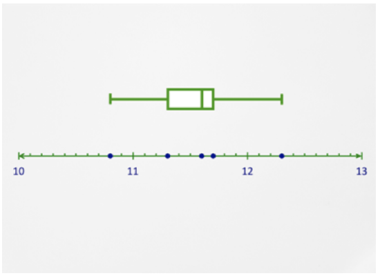
When the two outliers are removed, Sandra can see that most of the data is grouped closely together. Her time, 11.1, is still in the first quartile. However, her competition is tight because the rest of the team isn’t far behind.
Examples
Example 1
Earlier, you were given a problem about the books in the boxes. The number of books in each box on the truck is recorded. These numbers are:
15, 1, 20, 7, 15, 8, 3, 20, 8, 16, 3, 4, 13, 17, 20, 9, 6, 16, 22, 12, 6, 19, 7, 9, 10, 15, 9, 18, 19, 15, 14, 15, 2, 28, 10, 17, 7, 10, 8, 8
You need to:
a. Construct a box and whisker plot to represent the data.
b. What do you think is a “typical” number of books in a box? Justify your answer.
c. Are their outliers? Explain.
Let’s start with part a.
First, place the data in order.
1, 2, 3, 3, 4, 6, 6, 7, 7, 7, 8, 8, 8, 8, 9, 9, 9, 10, 10, 10, 12, 13, 14, 15, 15, 15, 15, 15, 16, 16, 17, 17, 18, 19, 19, 20, 20, 20, 22, 28
Next, draw a number line that includes the extremes.
The extreme maximum is 28 and the extreme minimum is 1.
The number line is drawn from 0 to 30.
Then, find the median and place this number on the number line.
The median is the middle data value. There are 40 data points. The 20th and 21st data values are 10 and 12. The median is 11.
Then, find the first and third quartiles and place these numbers on the number line.
Calculate the median of the two groups above and below the median of the data set.
Group 1: 1, 2, 3, 3, 4, 6, 6, 7, 7, 7, 8, 8, 8, 8, 9, 9, 9, 10, 10, 10
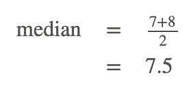
Group 2: 12, 13, 14, 15, 15, 15, 15, 15, 16, 16, 17, 17, 18, 19, 19, 20, 20, 20, 22, 28
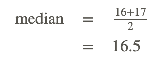
Then, draw boxes between the quartiles and the median.
Place the extremes, 1 and 28, on the numbers with points.
Finally draws whiskers from the quartiles to the extremes.
The diagram is below.

Let’s now do part b.
Any point within the box would be typical.
You could choose the median of 11 books as typical or even the mean of 12.
Finally, do part c.
An outlier is a data item that is far away from the general trend.
Twenty-eight is not a typical value as it is much larger than the others. It is an outlier.
Example 2
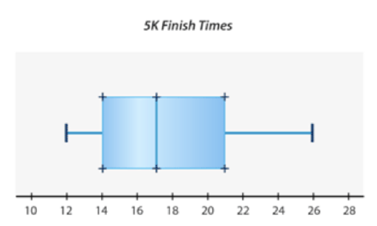
The town hall held its annual 5k run. Here are the times of the finishers: 12 minutes, 13 minutes, 14 minutes, 15 minutes, 16 minutes, 17 minutes, 18 minutes, 19 minutes, 21 minutes, 23 minutes and 26 minutes.
Create a box-and-whisker plot to show the data.
First, find the extremes in the data.
12, 13, 14, 15, 16, 17, 18, 19, 21, 23, 26
The extreme maximum is 26 and the extreme minimum is 12. The number line is drawn from 10 to 28.
Next, find the median and place this number on the number line.
The median is the middle data value. There are 11 data points. The median is 17.
Then, find the first and third quartiles and place these numbers on the number line.
Find the median of the two groups above and below the median of the data set.
Group 1: 12, 13, 14, 15, 16
Median = 14
Group 2: 18, 19, 21, 23, 26
Median = 21
Then, draw boxes between the quartiles and the median. Place the extremes, 12 and 26, on the numbers with points. Finally draw whiskers from the quartiles to the extremes.
The diagram is below.
Answer each question about box-and-whisker plots.
Example 3
What is a value called when it is found very far away from the median?
The answer is an outlier.
Example 4
Will removing an outlier change the median or the mean?
The answer is that it will change both.
The median value will be different, and the first and third quartile values will be affected because the outlier will not be calculated as part of the average.
Example 5
Does a box-and-whisker plot always have quartiles?
The answer is yes.
It is organized around the quartiles and the median.
Review
Define the following terms.
1. Box-whisker-plot
2. Quartiles
3. Median
4. Extremes
5. Interquartile Range
6. Outliers
Use the given box-and-whisker plot to answer the following questions.
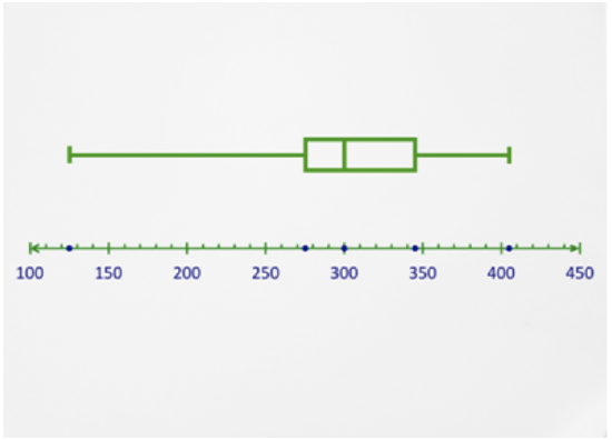
What is the median value?
8. Identify the quartiles.
9. Identify the interquartile range.
10. Identify any extremes.
11. Identify any outliers.
Use the data set to answer each question.
26, 27, 29, 30, 32, 35, 41, 42, 44
12. What is the median value?
13. Identify the median of the lower quartile.
14. Identify the median of the upper quartile.
15. Identify the lower extreme.
16. Identify the upper extreme.
Vocabulary
| Term | Definition |
|---|---|
| trace feature | The trace feature is a feature on the TI calculator that gives individual values to the five number summary of the box-and-whisker plot. |
Additional Resources
PLIX: Play, Learn, Interact, eXplore - Box-and-Whisker Plot: Babies in a Waiting Room
Video: Applications of Box an Whisker Plots Principles
Activities: Applications of Box-and-Whisker Plots Discussion Question
Lesson Plans: Creating Box and Whisker Plots with Technology Lesson Plan
Practice: Applications of Box-and-Whisker Plots
Real World: Counting Coral

