7.2: Simulation of Random Behavior and Probability Distributions
- Page ID
- 5735
\( \newcommand{\vecs}[1]{\overset { \scriptstyle \rightharpoonup} {\mathbf{#1}} } \)
\( \newcommand{\vecd}[1]{\overset{-\!-\!\rightharpoonup}{\vphantom{a}\smash {#1}}} \)
\( \newcommand{\id}{\mathrm{id}}\) \( \newcommand{\Span}{\mathrm{span}}\)
( \newcommand{\kernel}{\mathrm{null}\,}\) \( \newcommand{\range}{\mathrm{range}\,}\)
\( \newcommand{\RealPart}{\mathrm{Re}}\) \( \newcommand{\ImaginaryPart}{\mathrm{Im}}\)
\( \newcommand{\Argument}{\mathrm{Arg}}\) \( \newcommand{\norm}[1]{\| #1 \|}\)
\( \newcommand{\inner}[2]{\langle #1, #2 \rangle}\)
\( \newcommand{\Span}{\mathrm{span}}\)
\( \newcommand{\id}{\mathrm{id}}\)
\( \newcommand{\Span}{\mathrm{span}}\)
\( \newcommand{\kernel}{\mathrm{null}\,}\)
\( \newcommand{\range}{\mathrm{range}\,}\)
\( \newcommand{\RealPart}{\mathrm{Re}}\)
\( \newcommand{\ImaginaryPart}{\mathrm{Im}}\)
\( \newcommand{\Argument}{\mathrm{Arg}}\)
\( \newcommand{\norm}[1]{\| #1 \|}\)
\( \newcommand{\inner}[2]{\langle #1, #2 \rangle}\)
\( \newcommand{\Span}{\mathrm{span}}\) \( \newcommand{\AA}{\unicode[.8,0]{x212B}}\)
\( \newcommand{\vectorA}[1]{\vec{#1}} % arrow\)
\( \newcommand{\vectorAt}[1]{\vec{\text{#1}}} % arrow\)
\( \newcommand{\vectorB}[1]{\overset { \scriptstyle \rightharpoonup} {\mathbf{#1}} } \)
\( \newcommand{\vectorC}[1]{\textbf{#1}} \)
\( \newcommand{\vectorD}[1]{\overrightarrow{#1}} \)
\( \newcommand{\vectorDt}[1]{\overrightarrow{\text{#1}}} \)
\( \newcommand{\vectE}[1]{\overset{-\!-\!\rightharpoonup}{\vphantom{a}\smash{\mathbf {#1}}}} \)
\( \newcommand{\vecs}[1]{\overset { \scriptstyle \rightharpoonup} {\mathbf{#1}} } \)
\( \newcommand{\vecd}[1]{\overset{-\!-\!\rightharpoonup}{\vphantom{a}\smash {#1}}} \)
\(\newcommand{\avec}{\mathbf a}\) \(\newcommand{\bvec}{\mathbf b}\) \(\newcommand{\cvec}{\mathbf c}\) \(\newcommand{\dvec}{\mathbf d}\) \(\newcommand{\dtil}{\widetilde{\mathbf d}}\) \(\newcommand{\evec}{\mathbf e}\) \(\newcommand{\fvec}{\mathbf f}\) \(\newcommand{\nvec}{\mathbf n}\) \(\newcommand{\pvec}{\mathbf p}\) \(\newcommand{\qvec}{\mathbf q}\) \(\newcommand{\svec}{\mathbf s}\) \(\newcommand{\tvec}{\mathbf t}\) \(\newcommand{\uvec}{\mathbf u}\) \(\newcommand{\vvec}{\mathbf v}\) \(\newcommand{\wvec}{\mathbf w}\) \(\newcommand{\xvec}{\mathbf x}\) \(\newcommand{\yvec}{\mathbf y}\) \(\newcommand{\zvec}{\mathbf z}\) \(\newcommand{\rvec}{\mathbf r}\) \(\newcommand{\mvec}{\mathbf m}\) \(\newcommand{\zerovec}{\mathbf 0}\) \(\newcommand{\onevec}{\mathbf 1}\) \(\newcommand{\real}{\mathbb R}\) \(\newcommand{\twovec}[2]{\left[\begin{array}{r}#1 \\ #2 \end{array}\right]}\) \(\newcommand{\ctwovec}[2]{\left[\begin{array}{c}#1 \\ #2 \end{array}\right]}\) \(\newcommand{\threevec}[3]{\left[\begin{array}{r}#1 \\ #2 \\ #3 \end{array}\right]}\) \(\newcommand{\cthreevec}[3]{\left[\begin{array}{c}#1 \\ #2 \\ #3 \end{array}\right]}\) \(\newcommand{\fourvec}[4]{\left[\begin{array}{r}#1 \\ #2 \\ #3 \\ #4 \end{array}\right]}\) \(\newcommand{\cfourvec}[4]{\left[\begin{array}{c}#1 \\ #2 \\ #3 \\ #4 \end{array}\right]}\) \(\newcommand{\fivevec}[5]{\left[\begin{array}{r}#1 \\ #2 \\ #3 \\ #4 \\ #5 \\ \end{array}\right]}\) \(\newcommand{\cfivevec}[5]{\left[\begin{array}{c}#1 \\ #2 \\ #3 \\ #4 \\ #5 \\ \end{array}\right]}\) \(\newcommand{\mattwo}[4]{\left[\begin{array}{rr}#1 \amp #2 \\ #3 \amp #4 \\ \end{array}\right]}\) \(\newcommand{\laspan}[1]{\text{Span}\{#1\}}\) \(\newcommand{\bcal}{\cal B}\) \(\newcommand{\ccal}{\cal C}\) \(\newcommand{\scal}{\cal S}\) \(\newcommand{\wcal}{\cal W}\) \(\newcommand{\ecal}{\cal E}\) \(\newcommand{\coords}[2]{\left\{#1\right\}_{#2}}\) \(\newcommand{\gray}[1]{\color{gray}{#1}}\) \(\newcommand{\lgray}[1]{\color{lightgray}{#1}}\) \(\newcommand{\rank}{\operatorname{rank}}\) \(\newcommand{\row}{\text{Row}}\) \(\newcommand{\col}{\text{Col}}\) \(\renewcommand{\row}{\text{Row}}\) \(\newcommand{\nul}{\text{Nul}}\) \(\newcommand{\var}{\text{Var}}\) \(\newcommand{\corr}{\text{corr}}\) \(\newcommand{\len}[1]{\left|#1\right|}\) \(\newcommand{\bbar}{\overline{\bvec}}\) \(\newcommand{\bhat}{\widehat{\bvec}}\) \(\newcommand{\bperp}{\bvec^\perp}\) \(\newcommand{\xhat}{\widehat{\xvec}}\) \(\newcommand{\vhat}{\widehat{\vvec}}\) \(\newcommand{\uhat}{\widehat{\uvec}}\) \(\newcommand{\what}{\widehat{\wvec}}\) \(\newcommand{\Sighat}{\widehat{\Sigma}}\) \(\newcommand{\lt}{<}\) \(\newcommand{\gt}{>}\) \(\newcommand{\amp}{&}\) \(\definecolor{fillinmathshade}{gray}{0.9}\)Use Simulations to Explore Experimental Probability

CK-12 Foundation - CK-12 Foundation
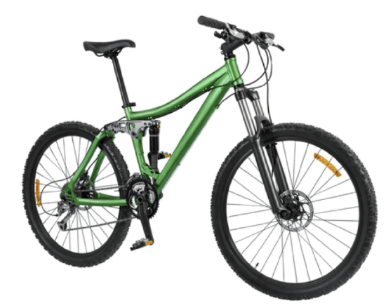
Terry stood in front of the window and looked at the bicycle. It was perfect. She had debated all of the different options that she could have and still she thought that the one in the window of the bike shop was the perfect one for her.
“I have to have it,” she said smiling.
“I guess you made up your mind,” Casey said.
“Yes, imagine if we had asked all of our friends which bike I should get, we would have had a ton of different answers,” Terry said.
Terry is correct there would have been a lot of answers to keep track and tally.
Design a simulation where Terry would have surveyed her classmates and figured out the probability that she would have selected this bike out of the other 16 options.
In this concept, you will learn to use simulations to explore experimental probability.
Simulations
A simulation is a way of collecting probability data using actual objects, such as coins, spinners, and cards.
Let’s look at an example.
Conduct a simulation to see how many times heads comes up when you flip a coin 50 times.
First, make a table like the one below. Conduct your simulation in groups of 10 flips. Leave lots of room to tally your results. Write in a prediction of how many times heads will turn up.
| Trial | 1 | 2 | 3 | 4 | 5 | Prediction | Total |
| Tally | X | X | |||||
| Heads | 25 | ||||||
| Total Flips | 50 |
Second, begin conducting your simulation. Tally your results. Some sample data is shown. Remember, this is a sample and not actual data.
| Trial | 1 | 2 | 3 | 4 | 5 | Prediction | Total |
| Tally | |||| | ||| | X | X | |||
| Heads | 25 | ||||||
| Total Flips | 10 | 10 | 10 | 10 | 10 | 50 |
Then, fill in the rest of your table. Here is what your completed table might look like.
| Trial | 1 | 2 | 3 | 4 | 5 | Prediction | Total |
| Tally | |||| | ||| | X | X | |||
| Heads | 4 | 5 | 3 | 6 | 5 | 25 | 23 |
| Total Flips | 10 | 10 | 10 | 10 | 10 | 50 | 50 |
Now that you are set up and understand the process, run the simulations and solve the problems that follow. Record your data. Make sure you make a table and predictions for each simulation.
Let’s look at another example.
Run a simulation of 60 coin flips to see how frequently tails turns up.
- How many times did you predict tails would occur? How many times did it actually occur?
- How well did your data agree with your prediction? Explain.
Work on this simulation with a partner. Record your data and then discuss your answers.
Many calculators and websites have random number generators and other features that can be used to generate data for simulations. Here you will use the website http://www.random.org to run a coin flipping simulation.
First, make a table for collecting coin flip data like the one shown. Fill in your prediction. You won’t need to tally data here –the computer will do it for you.
| Trial | 1 | 2 | 3 | 4 | 5 | 6 | 7 | 8 | 9 | 10 | Prediction | Total |
| Heads | ||||||||||||
| Total Flips |
Next, open the webpage http://www.random.org/. Click on “coin flipper.” Here you selected 10 as the number of coins to flip on each trial. Click on “Flip coin(s)”. Record the data in the table. Sample data collected from the website is shown below.
| Trial | 1 | 2 | 3 | 4 | 5 | 6 | 7 | 8 | 9 | 10 | Prediction | Total |
| Heads | 6 | 4 | 6 | 2 | 7 | 6 | 6 | 5 | 5 | 5 | 50 | 52 |
| Total Flips | 10 | 10 | 10 | 10 | 10 | 10 | 10 | 10 | 10 | 10 | 100 | 100 |
Then, analyze your data. How accurate was your prediction?
The prediction was that there is a 50% chance of flipping heads. After doing 100 trials, the simulation showed that 52% of the time, the coin flipped heads.
Examples
Example 1
Earlier, you were given a problem about Terry and the bike. Terry needs to conduct a simulation to conduct a survey of her classmates on what bike they would recommend of the 16 different options.
First, to accomplish this task, Terry could write out all of the 16 options for bicycles. Then she could go around and ask her friends to rate the bikes 1, 2 or 3. One being the first choice etc.
Next, Terry could calculate her scores and narrow it down to the bikes that received the most votes. The bicycle that was selected the most times would be the winning bike.
Example 2
Jessie decided to conduct an experiment with a spinner. The spinner is divided into four colors: red, blue, orange and green. Jessie predicted that out of 30 spins that the spinner would be red 10% of the time.
She conducted the experiment and the spinner was red four times. Is her prediction correct?
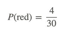
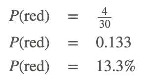
First, to figure this out, you must first write a probability and then compare it to the 10% that Jessie predicted. The actual result is that the spinner was red 4 out of 30 times.

Second, convert to a percent.

The answer is 13.3%.
Jessie’s prediction was too low. The actual result was higher than 10%.
Example 3
Is the following statement true or false?
A simulation is an experiment.
This statement is true.
Example 4
Is the following statement true or false?
To explore experimental probability, you could simply spin a spinner one time.
This statement is false. You need to have more than one trial in an experiment to be exploring experimental probability.
Example 5
Is the following statement true or false?
To use a coin in a simulation, you would need to flip the coin many, many times.
This statement is true.
Review
Run a simulation using playing cards. Make a stack of the Ace, Jack, King, Queen, and Ten of each suit. Predict how frequently an Ace will turn up. Run 60 trials in groups of 10. Return the card to the deck and shuffle after you choose each card. Use a table like the one below.
| Trial | 1 | 2 | 3 | 4 | 5 | 6 | Prediction | Total |
| Tally | ||||||||
| Ace | ||||||||
| Total tosses | 10 | 10 | 10 | 10 | 10 | 10 |
- How many times did you predict an Ace would occur? How many times did it actually occur?
- How well does your data agree with your prediction?
Run a simulation using playing cards. Make a stack of the Ace, Jack, King, Queen, and Ten of each suit. Predict how frequently a King, a Queen and a Jack will turn up. Run 60 trials in groups of 10. Return the card to the deck and shuffle after you choose each card. Use a table like the one below.
| Trial | 1 | 2 | 3 | 4 | 5 | 6 | Prediction | Total |
| Tally | ||||||||
| Ace | ||||||||
| Total tosses | 10 | 10 | 10 | 10 | 10 | 10 |
3. How many times did you predict an King would occur? How many times did it actually occur?
4. How many times did you predict a Jack would occur? How many times did it actually occur?
5. How many times did you predict a Queen would occur? How many times did it actually occur?
6. How well does your data agree with your prediction?
Run a simulation of 72 number cube tosses in groups of 12 to see how frequently 4 or 5 turns up. Use a table like the one below.
| Trial | 1 | 2 | 3 | 4 | 5 | 6 | Prediction | Total |
| Tally | ||||||||
| 4 Or 5 | ||||||||
| Total tosses | 12 | 12 | 12 | 12 | 12 | 12 |
7. How many times did you predict 4 or 5 would occur? How many times did it actually occur?
8. How well does your data agree with your prediction?
9. Try another group of 36 tosses. Add your results of 36 tosses to your previous 72 tosses to make 108 total tosses. How well did your data now agree with your prediction? Explain.
Use http://www.random.org for each simulation. Run a number cube simulation to see how many times each number on the cube comes up. In http://www.random.org/, click on the link that reads “dice roller”. Choose 12 for the number of number cubes (dice) you want to roll. Set up a table like the one below to have a total of 96 rolls.
Tally up the number of 1s, 2s, 3s, 4s, 5s, and 6s that turn up and record them in the table. Keep rolling until you have a total of 96 rolls.
| Number |
1 |
2 |
3 |
4 |
5 |
6 |
Total |
| Tally | |||||||
| Total | 96 | ||||||
| Prediction | 16 | 16 | 16 | 16 | 16 | 16 | 96 |
10. How many times did you predict each number on the number cube would appear in 96 rolls?
11. How many times did it actually appear?
12. How well does your data agree with your prediction?
13. Try an additional 96 rolls. How did the additional data change your results? Explain.
Now design your own simulation and use a spinner or two number cubes.
Vocabulary
| Term | Definition |
|---|---|
| Simulation | A way of collecting data using objects such as spinners, coins or cards. |
Additional Resources
PLIX: Play, Learn, Interact, eXplore - Roll One!
Video: Probability Part 3
Practice: Simulation of Random Behavior and Probability Distributions


