7.8: Central Limit Theorem
- Page ID
- 5741
\( \newcommand{\vecs}[1]{\overset { \scriptstyle \rightharpoonup} {\mathbf{#1}} } \)
\( \newcommand{\vecd}[1]{\overset{-\!-\!\rightharpoonup}{\vphantom{a}\smash {#1}}} \)
\( \newcommand{\id}{\mathrm{id}}\) \( \newcommand{\Span}{\mathrm{span}}\)
( \newcommand{\kernel}{\mathrm{null}\,}\) \( \newcommand{\range}{\mathrm{range}\,}\)
\( \newcommand{\RealPart}{\mathrm{Re}}\) \( \newcommand{\ImaginaryPart}{\mathrm{Im}}\)
\( \newcommand{\Argument}{\mathrm{Arg}}\) \( \newcommand{\norm}[1]{\| #1 \|}\)
\( \newcommand{\inner}[2]{\langle #1, #2 \rangle}\)
\( \newcommand{\Span}{\mathrm{span}}\)
\( \newcommand{\id}{\mathrm{id}}\)
\( \newcommand{\Span}{\mathrm{span}}\)
\( \newcommand{\kernel}{\mathrm{null}\,}\)
\( \newcommand{\range}{\mathrm{range}\,}\)
\( \newcommand{\RealPart}{\mathrm{Re}}\)
\( \newcommand{\ImaginaryPart}{\mathrm{Im}}\)
\( \newcommand{\Argument}{\mathrm{Arg}}\)
\( \newcommand{\norm}[1]{\| #1 \|}\)
\( \newcommand{\inner}[2]{\langle #1, #2 \rangle}\)
\( \newcommand{\Span}{\mathrm{span}}\) \( \newcommand{\AA}{\unicode[.8,0]{x212B}}\)
\( \newcommand{\vectorA}[1]{\vec{#1}} % arrow\)
\( \newcommand{\vectorAt}[1]{\vec{\text{#1}}} % arrow\)
\( \newcommand{\vectorB}[1]{\overset { \scriptstyle \rightharpoonup} {\mathbf{#1}} } \)
\( \newcommand{\vectorC}[1]{\textbf{#1}} \)
\( \newcommand{\vectorD}[1]{\overrightarrow{#1}} \)
\( \newcommand{\vectorDt}[1]{\overrightarrow{\text{#1}}} \)
\( \newcommand{\vectE}[1]{\overset{-\!-\!\rightharpoonup}{\vphantom{a}\smash{\mathbf {#1}}}} \)
\( \newcommand{\vecs}[1]{\overset { \scriptstyle \rightharpoonup} {\mathbf{#1}} } \)
\( \newcommand{\vecd}[1]{\overset{-\!-\!\rightharpoonup}{\vphantom{a}\smash {#1}}} \)
\(\newcommand{\avec}{\mathbf a}\) \(\newcommand{\bvec}{\mathbf b}\) \(\newcommand{\cvec}{\mathbf c}\) \(\newcommand{\dvec}{\mathbf d}\) \(\newcommand{\dtil}{\widetilde{\mathbf d}}\) \(\newcommand{\evec}{\mathbf e}\) \(\newcommand{\fvec}{\mathbf f}\) \(\newcommand{\nvec}{\mathbf n}\) \(\newcommand{\pvec}{\mathbf p}\) \(\newcommand{\qvec}{\mathbf q}\) \(\newcommand{\svec}{\mathbf s}\) \(\newcommand{\tvec}{\mathbf t}\) \(\newcommand{\uvec}{\mathbf u}\) \(\newcommand{\vvec}{\mathbf v}\) \(\newcommand{\wvec}{\mathbf w}\) \(\newcommand{\xvec}{\mathbf x}\) \(\newcommand{\yvec}{\mathbf y}\) \(\newcommand{\zvec}{\mathbf z}\) \(\newcommand{\rvec}{\mathbf r}\) \(\newcommand{\mvec}{\mathbf m}\) \(\newcommand{\zerovec}{\mathbf 0}\) \(\newcommand{\onevec}{\mathbf 1}\) \(\newcommand{\real}{\mathbb R}\) \(\newcommand{\twovec}[2]{\left[\begin{array}{r}#1 \\ #2 \end{array}\right]}\) \(\newcommand{\ctwovec}[2]{\left[\begin{array}{c}#1 \\ #2 \end{array}\right]}\) \(\newcommand{\threevec}[3]{\left[\begin{array}{r}#1 \\ #2 \\ #3 \end{array}\right]}\) \(\newcommand{\cthreevec}[3]{\left[\begin{array}{c}#1 \\ #2 \\ #3 \end{array}\right]}\) \(\newcommand{\fourvec}[4]{\left[\begin{array}{r}#1 \\ #2 \\ #3 \\ #4 \end{array}\right]}\) \(\newcommand{\cfourvec}[4]{\left[\begin{array}{c}#1 \\ #2 \\ #3 \\ #4 \end{array}\right]}\) \(\newcommand{\fivevec}[5]{\left[\begin{array}{r}#1 \\ #2 \\ #3 \\ #4 \\ #5 \\ \end{array}\right]}\) \(\newcommand{\cfivevec}[5]{\left[\begin{array}{c}#1 \\ #2 \\ #3 \\ #4 \\ #5 \\ \end{array}\right]}\) \(\newcommand{\mattwo}[4]{\left[\begin{array}{rr}#1 \amp #2 \\ #3 \amp #4 \\ \end{array}\right]}\) \(\newcommand{\laspan}[1]{\text{Span}\{#1\}}\) \(\newcommand{\bcal}{\cal B}\) \(\newcommand{\ccal}{\cal C}\) \(\newcommand{\scal}{\cal S}\) \(\newcommand{\wcal}{\cal W}\) \(\newcommand{\ecal}{\cal E}\) \(\newcommand{\coords}[2]{\left\{#1\right\}_{#2}}\) \(\newcommand{\gray}[1]{\color{gray}{#1}}\) \(\newcommand{\lgray}[1]{\color{lightgray}{#1}}\) \(\newcommand{\rank}{\operatorname{rank}}\) \(\newcommand{\row}{\text{Row}}\) \(\newcommand{\col}{\text{Col}}\) \(\renewcommand{\row}{\text{Row}}\) \(\newcommand{\nul}{\text{Nul}}\) \(\newcommand{\var}{\text{Var}}\) \(\newcommand{\corr}{\text{corr}}\) \(\newcommand{\len}[1]{\left|#1\right|}\) \(\newcommand{\bbar}{\overline{\bvec}}\) \(\newcommand{\bhat}{\widehat{\bvec}}\) \(\newcommand{\bperp}{\bvec^\perp}\) \(\newcommand{\xhat}{\widehat{\xvec}}\) \(\newcommand{\vhat}{\widehat{\vvec}}\) \(\newcommand{\uhat}{\widehat{\uvec}}\) \(\newcommand{\what}{\widehat{\wvec}}\) \(\newcommand{\Sighat}{\widehat{\Sigma}}\) \(\newcommand{\lt}{<}\) \(\newcommand{\gt}{>}\) \(\newcommand{\amp}{&}\) \(\definecolor{fillinmathshade}{gray}{0.9}\)The Central Limit Theorem
In the previous lesson, you learned that sampling is an important tool for determining the characteristics of a population. Although the parameters of the population (mean, standard deviation, etc.) were unknown, random sampling was used to yield reliable estimates of these values. The estimates were plotted on graphs to provide a visual representation of the distribution of the sample means for various sample sizes. It is now time to define some properties of a sampling distribution of sample means and to examine what we can conclude about the entire population based on these properties.
Central Limit Theorem
The Central Limit Theorem is a very important theorem in statistics. It basically confirms what might be an intuitive truth to you: that as you increase the sample size for a random variable, the distribution of the sample means better approximates a normal distribution.
Before going any further, you should become familiar with (or reacquaint yourself with) the symbols that are commonly used when dealing with properties of the sampling distribution of sample means. These symbols are shown in the table below:
| Population Parameter | Sample Statistic | Sampling Distribution | |
|---|---|---|---|
| Mean | μ | x̄ | μx̄ |
| Standard Deviation | σ | s | Sx̄ or σx̄ |
| Size | N | n |
As the sample size, n, increases, the resulting sampling distribution would approach a normal distribution with the same mean as the population and with σx̄=σ/n.5. The notation σx¯ reminds you that this is the standard deviation of the distribution of sample means and not the standard deviation of a single observation.
The Central Limit Theorem states the following:
If samples of size n are drawn at random from any population with a finite mean and standard deviation, then the sampling distribution of the sample means, x̄, approximates a normal distribution as n increases.
The mean of this sampling distribution approximates the population mean, and the standard deviation of this sampling distribution approximates the standard deviation of the population divided by the square root of the sample size: μx̄=μ and σx̄=σ/n0.5.
These properties of the sampling distribution of sample means can be applied to determining probabilities. If the sample size is sufficiently large (>30), the sampling distribution of sample means can be assumed to be approximately normal, even if the population is not normally distributed.
Applying the Central Limit Theorem
1. Suppose you wanted to answer the question, “What is the probability that a random sample of 20 families in Canada will have an average of 1.5 pets or fewer?” where the mean of the population is 0.8 and the standard deviation of the population is 1.2.
For the sampling distribution, μx̄=μ=0.8 and σx̄=σ/n.5=1.2200.5=0.268.
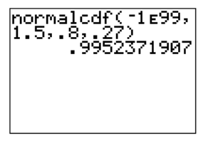
We can use a graphing calculator as follows:

Therefore, the probability that the sample mean will be below 1.5 is 0.9952. In other words, with a random sample of 20 families, it is almost definite that the average number of pets per family will be less than 1.5.
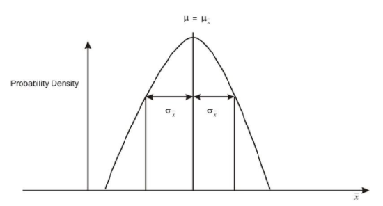
The properties associated with the Central Limit Theorem are displayed in the diagram below:

The vertical axis now reads probability density, rather than frequency, since frequency can only be used when you are dealing with a finite number of sample means. Sampling distributions, on the other hand, are theoretical depictions of an infinite number of sample means, and probability density is the relative density of the selections from within this set.
The question indicates that multiple samples of size 40 are being collected from a known population, multiple sample means are being calculated, and then the sampling distribution of the sample means is being studied. Therefore, an understanding of the Central Limit Theorem is necessary to answer the question.
2. A random sample of size 40 is selected from a known population with a mean of 23.5 and a standard deviation of 4.3. Samples of the same size are repeatedly collected, allowing a sampling distribution of sample means to be drawn.
a) What is the expected shape of the resulting distribution?
The sampling distribution of the sample means will be approximately bell-shaped.
b) Where is the sampling distribution of sample means centered?
The sampling distribution of the sample means will be centered about the population mean of 23.5.
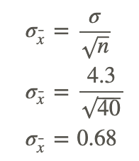
c) What is the approximate standard deviation of the sample means?
The approximate standard deviation of the sample means is 0.68, which can be calculated as shown below:

Calculations Involving Sample Means
Multiple samples with a sample size of 40 are taken from a known population, where μ=25 and σ=4. The following chart displays the sample means:
| 25 | 25 | 26 | 26 | 26 | 24 | 25 | 25 | 24 | 25 |
| 26 | 25 | 26 | 25 | 24 | 25 | 25 | 25 | 25 | 25 |
| 24 | 24 | 24 | 24 | 26 | 26 | 26 | 25 | 25 | 25 |
| 25 | 25 | 24 | 24 | 25 | 25 | 25 | 24 | 25 | 25 |
| 25 | 24 | 25 | 25 | 24 | 26 | 24 | 26 | 24 | 26 |
1. What is the population mean?
The population mean of 25 was given in the question:
μ=25.
2. Using technology, determine the mean of the sample means.
The mean of the sample means is 24.94 and is determined by using '1 Vars Stat' on the TI-83/84 calculator:
μx̄=24.94.
3. What is the population standard deviation?
The population standard deviation of 4 was given in the question:
σ=4.
4. Using technology, determine the standard deviation of the sample means.
The standard deviation of the sample means is 0.71 and is determined by using '1 Vars Stat' on the TI-83/84 calculator:
Sx̄=0.71.
Note that the Central Limit Theorem states that the standard deviation should be approximately
440.5=0.63.
5. As the sample size increases, what value will the mean of the sample means approach?
The mean of the sample means will approach 25 and is determined by a property of the Central Limit Theorem:
μx̄=25.
6. As the sample size increases, what value will the standard deviation of the sample means approach?
The standard deviation of the sample means will approach 4/n.5 and is determined by a property of the Central Limit Theorem: σx̄=4/n.5.
Examples
The weights of women in a particular age group have mean of 130 pounds and standard deviation of 18 pounds. Assume the weights are normally distributed.
Example 1
For a randomly selected group of women what is the standard deviation of the sampling distribution of the possible sample means?
σx̄=183=6
Example 2
For a randomly selected group of women what is the standard deviation of the sampling distribution of possible sample means?
σx̄=189=2
Example 3
How does sample size affect the standard deviation of the sampling distribution of possible means?
As sample size increases the standard deviation of the sampling distribution of possible means decreases. You divide by the square root of the sample size and as you divide by a larger number, the value of the fraction decreases.
Review
- The lifetimes of a certain type of calculator battery are normally distributed. The mean lifetime is 400 days, with a standard deviation of 50 days. For a sample of 6000 new batteries, determine how many batteries will last:
- between 360 and 460 days.
- more than 320 days.
- less than 280 days.
- How does sample size affect the variation in sample results?
- For each of the following situations determine if the Central Limit Theorem can be applied:
- In the world populations, normal body temperature follows a normal distribution with mean = 98.6 degrees F and a standard deviation of 0.6. The mean body temperature will be determined for a randomly selected group of 14 individuals.
- Mean number of songs on a student’s IPOD will be determined for a randomly selected group of 10 students. In the college population it is known that the number of songs on a student’s ipod is skewed to the left.
- Now assume that you are randomly selecting 800 students to determine the mean number of songs on the ipod.
- You randomly draw 100 samples of 10 subjects and calculate the mean for each of the samples. You plot the sample means. What is the name of the distribution that you have created?
- A scientist plots a set of sample means drawn from 200 samples, each of 40 subjects. What should her distribution look like? Explain.
- The weights of people in a certain population are normally distributed with a mean of 160 pounds and a standard deviation of 27 pounds. Consider samples of size 7. State whether the distribution of is normal or approximately normal and give its mean and standard deviation.
- The mean annual income for adult men in one city is $45,632 and the standard deviation of the incomes is $4500. Consider samples of size 53. State whether the distribution of is normal or approximately normal and give its mean and standard deviation.
- If a random sample of 1,000 was taken from a database and a histogram was made of the data which of the following is likely to be true:
- the histogram will look approximately like a normal distribution because the sample size is large, and the Central Limit Theorem applies.
- The histogram will look approximately like a normal distribution because the number of samples taken is large and the Central Limit Theorem applies.
- The histogram will be skewed to the left.
- The histogram will be skewed to the right.
- Suppose we compare 2 random samples taken from the same populations. Sample A is a random sample of 100 subjects and sample B is a random sample of 1000 subjects. What can be said about the relationship between the sample standard deviations in sample A relative to the sample standard deviation of sample B?
- A sample of 500 subjects is a skewed distribution. The sampling distribution of the sample mean
- Will be approximately normally distributed
- Will be skewed
- Not enough information to determine
- Two graduate students are each doing a study and are pulling their samples from the same population. The first investigator takes a sample of 100 and the second takes a sample of 2,000.
- Which student will tend to get the larger standard deviation in his/her sample?
- Which student will get a larger standard error of the mean? Or can it not be determined?
- The mean annual income for adult men in one city is $28,520 and the standard deviation of the incomes is $5000. The distribution of incomes is skewed to the left. Determine the sampling distribution of the mean for samples of size 43.
- Approximately normal, mean = $28,500, standard deviation $762.
- Normal, mean = $28,500, standard deviation = $762.
- Normal, mean = $28,500, standard deviation = $116
- Approximately normal, mean = $28,5000, standard deviation = $5,000.
- The Central Limit Theorem says the sampling distribution of the sample mean is approximately normal under certain conditions. What is a necessary condition for the Central Limit Theorem to be used?
- The population size must e large (at least 30)
- The population from which we are sampling must not be normally distributed.
- The population from which we are sampling must be normally distributed.
- The sample size must be large (at least 30).
- True or False: (explain) The Central Limit Theorem guarantees that the population is normal whenever n is sufficiently large.
- The average life of an electric rice cooker is 5 years, with a standard deviation of 1 year. Assume the lives of these cookers follow a normal distribution. Find
- The probability that the mean life of a random sample of 9 machines falls between 5.7 and 8.1 years.
- The value of to the left of which 85% of the means computed from random samples of size 9 would fall.
- True or False? The mean height for a population is 67 inches and the standard deviation is 4 inches. Let denote the mean height for a sample of people picked randomly from the population. True or False: The standard deviation of for samples of size 30 or greater is the standard deviation of for samples of size 20?
- Suppose you select a random sample of 200 student responses to the question, “how many hours did you study last night?” Suppose that in a large population of students the mean number of hours of study the previous night was hours with a standard deviation of hours.
- What is the value of the mean of the sampling distribution of possible sample means?
- Calculate the standard deviation of the sampling distribution of possible sample means.
- Consider. For the 200 students randomly selected find the values of and using the empirical rule.
- For the same 200 randomly selected students, using the empirical rule, find the interval within which 95% of the mean number of hours of study will fall.
- The amount of time it takes a student to walk from her home to class has a skewed right distribution with a mean of 18 minutes and a standard deviation of 1.8 minutes. If data were collected from 30 randomly selected walks, describe the sampling distribution of the sample mean.
- The amount of soda a dispensing machine pours into a 24-ounce can of soda follows a normal distribution with a mean of 24.05 ounces and a standard deviation of .02 ounces. Suppose the quality control department at the soda plant sampled 100 sodas and found the average amount of soda in the cans was 24 ounces of soda. What should the quality control department recommend to the management of the plant?
Vocabulary
| Term | Definition |
|---|---|
| Central Limit Theorem | The Central Limit Theorem states that if samples are drawn at random from any population with a finite mean and standard deviation, then the sampling distribution of the sample means approximates a normal distribution as the sample size increases beyond 30. |
| sampling distribution of the sample means | The sampling distribution of the sample mean is the distribution that describes the spread of the means of multiple samples from the same population. |
Additional Resouces
Video: Sampling Distribution of the Sample Mean
Practice: Central Limit Theorem
Real World: Violent Times

