10.4: Multiple Regression

Multiple Regression

We have learned a bit about examining the relationship between two variables by calculating the correlation coefficient and the linear regression line. But, as we all know, often times we work with more than two variables. For example, what happens if we want to examine the impact that class size and number of faculty members have on a university's ranking. Since we are taking multiple variables into account, the linear regression model just won’t work. In multiple linear regression, scores for one variable are predicted (in this example, a university's ranking) using multiple predictor variables (class size and number of faculty members).

Another common use of multiple regression models is in the estimation of the selling price of a home. There are a number of variables that go into determining how much a particular house will cost, including the square footage, the number of bedrooms, the number of bathrooms, the age of the house, the neighborhood, and so on. Analysts use multiple regression to estimate the selling price in relation to all of these different types of variables.

In this Concept, we will examine the components of a multiple regression equation, calculate an equation using technological tools, and use this equation to test for significance in order to evaluate a hypothesis.

Understanding a Multiple Regression Equation

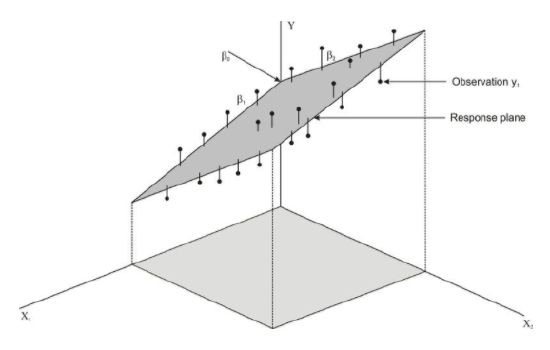
If we were to try to draw a multiple regression model, it would be a bit more difficult than drawing a model for linear regression. Let’s say that we have two predictor variables, X₁ and X₂, that are predicting the desired variable, Y. The regression equation would be as follows:

Ŷ =b₁X₁+b₂X₂+a

When there are two predictor variables, the scores must be plotted in three dimensions (see figure below). When there are more than two predictor variables, we would continue to plot these in multiple dimensions. Regardless of how many predictor variables there are, we still use the least squares method to try to minimize the distance between the actual and predicted values.

When predicting values using multiple regression, we first use the standard score form of the regression equation, which is shown below:

Ŷ =β₁X₁+β₂X₂+…+β_iX_i

where:

Ŷ is the predicted variable, or criterion variable.

β_i is the ith regression coefficient.

X_i is the ith predictor variable.

To solve for the regression and constant coefficients, we need to determine multiple correlation coefficients, r, and coefficients of determination, also known as proportions of shared variance, r₂. In the linear regression model, we measured r₂ by adding the squares of the distances from the actual points to the points predicted by the regression line. So what does r₂ look like in the multiple regression model? Let’s take a look at the figure above. Essentially, like in the linear regression model, the theory behind the computation of a multiple regression equation is to minimize the sum of the squared deviations from the observations to the regression plane.

In most situations, we use a computer to calculate the multiple regression equation and determine the coefficients in this equation. We can also do multiple regression on a TI-83/84 calculator. (This program can be downloaded.)

Technology Note: Multiple Regression Analysis on the TI-83/84 Calculator

Download a program for multiple regression analysis on the TI-83/84 calculator by first clicking on the link above.

It is helpful to explain the calculations that go into a multiple regression equation so we can get a better understanding of how this formula works.

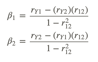
After we find the correlation values, r, between the variables, we can use the following formulas to determine the regression coefficients for the predictor variables, X₁ and X₂:

where:

β₁ is the correlation coefficient for X₁.

β₂ is the correlation coefficient for X₂.

r_Y1 is the correlation between the criterion variable, Y, and the first predictor variable, X₁.

r_Y2 is the correlation between the criterion variable, Y, and the second predictor variable, X₂.

r₁₂ is the correlation between the two predictor variables, X₁ and X₂.

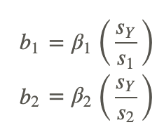
After solving for the beta coefficients, we can then compute the b coefficients by using the following formulas:

where:

s_Y is the standard deviation of the criterion variable, Y.

s₁ is the standard deviation of the particular predictor variable (1 for the first predictor variable, 2 for the second, and so on).

After solving for the regression coefficients, we can finally solve for the regression constant by using the formula shown below, where k is the number of predictor variables:

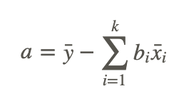
Again, since these formulas and calculations are extremely tedious to complete by hand, we usually use a computer or a TI-83/84 calculator to solve for the coefficients in a multiple regression equation.

Calculating a Multiple Regression Equation using Technological Tools

As mentioned, there are a variety of technological tools available to calculate the coefficients in a multiple regression equation. When using a computer, there are several programs that help us calculate the multiple regression equation, including Microsoft Excel, the Statistical Analysis Software (SAS), and the Statistical Package for the Social Sciences (SPSS). Each of these programs allows the user to calculate the multiple regression equation and provides summary statistics for each of the models.

For the purposes of this lesson, we will synthesize summary tables produced by Microsoft Excel to solve problems with multiple regression equations. While the summary tables produced by the different technological tools differ slightly in format, they all provide us with the information needed to build a multiple regression equation, conduct hypothesis tests, and construct confidence intervals. Let’s take a look at an example of a summary statistics table so we get a better idea of how we can use technological tools to build multiple regression equations.

Suppose we want to predict the amount of water consumed by football players during summer practices. The football coach notices that the water consumption tends to be influenced by the time that the players are on the field and by the temperature. He measures the average water consumption, temperature, and practice time for seven practices and records the following data:

Temperature (degrees F)	Practice Time (hrs)	H2O Consumption (in ounces)
75	1.85	16
83	1.25	20
85	1.5	25
85	1.75	27
92	1.15	32
97	1.75	48
99	1.6	48

Figure: Water consumption by football players compared to practice time and temperature.

Technology Note: Using Excel for Multiple Regression

• Copy and paste the table into an empty Excel worksheet.
• Click the Data choice on the toolbar, then select ’Data Analysis,’ and then choose ’Regression’ from the list that appears (Note, if Data Analysis does not appear as a choice on your Data page need to follow the add-in instructions below).
• Place the cursor in the ’Input Y range’ field and select the third column.
• Place the cursor in the ’Input X range’ field and select the first and second columns.
• Place the cursor in the ’Output Range’ field and click somewhere in a blank cell below and to the left of the table.
• Click ’Labels’ so that the names of the predictor variables will be displayed in the table.
• Click ’OK’, and the results shown below will be displayed.

Note: In Excel 2007, to add Data Analysis to your Data page, perform the following functions. Click the Microsoft Office Button in the upper left, then click on Excel Options. Click on Add-ins, then highlight the Analysis ToolPak, click Go, make sure the Analysis ToolPak box is checked off, and then click OK. The Data Analysis choice should now appear on your Excel Data page. Follow the remaining instructions above.

SUMMARY OUTPUT

Regression Statistics

Df	SS	MS	F	Significance F
Regression	2	970.6583	485.3291	313.1723	4.03E-05
Residual	4	6.198878	1.549719
Total	6	976.8571

	Coefficients	Standard Error	t Stat	P-value	Lower 95%	Upper 95%
Intercept	−121.655	6.540348	−18.6007	4.92e-05	−139.814	−103.496
Temperature	1.512364	0.060771	24.88626	1.55E-05	1.343636	1.681092
Practice Time	12.53168	1.93302	6.482954	0.002918	7.164746	17.89862

In this example, we have a number of summary statistics that give us information about the regression equation. As you can see from the results above, we have the regression coefficient and standard error for each variable, as well as the value of r2. We can take all of the regression coefficients and put them together to make our equation.

Using the results above, our regression equation would be Ŷ =−121.66+1.51(Temperature)+12.53(Practice Time).

Each of the regression coefficients tells us something about the relationship between the predictor variable and the predicted outcome. The temperature coefficient of 1.51 tells us that for every 1.0-degree increase in temperature, we predict there to be an increase of 1.5 ounces of water consumed, if we hold the practice time constant. Similarly, we find that with every one-hour increase in practice time, we predict players will consume an additional 12.53 ounces of water, if we hold the temperature constant. That equates to about 2.1 extra ounces of water for every 10 minutes increase in practice time.

With a value of 0.99 for r₂, we can conclude that approximately 99% of the variance in the outcome variable, Y, can be explained by the variance in the combined predictor variables. With a value of 0.99 for r₂, we can conclude that almost all of the variance in water consumption is attributed to the variance in temperature and practice time.

Testing for Significance to Evaluate a Hypothesis, the Standard Error of a Coefficient, and Constructing Confidence Intervals

When we perform multiple regression analysis, we are essentially trying to determine if our predictor variables explain the variation in the outcome variable, Y. When we put together our final equation, we are looking at whether or not the variables explain most of the variation, r2, and if this value of r2 is statistically significant. We can use technological tools to conduct a hypothesis test, testing the significance of this value of r2, and construct confidence intervals around these results.

Hypothesis Testing

When we conduct a hypothesis test, we test the null hypothesis that the multiple r-value in the population equals zero, or H0:rpop=0. Under this scenario, the predicted values, or fitted values, would all be very close to the mean, and the deviations, Ŷ −Y¯, and the sum of the squares would be close to 0. Therefore, we want to calculate a test statistic (in this case, the F-statistic) that measures the correlation between the predictor variables. If this test statistic is beyond the critical values and the null hypothesis is rejected, we can conclude that there is a nonzero relationship between the criterion variable, Y, and the predictor variables. When we reject the null hypothesis, we can say something like, “The probability that r2 having the value obtained would have occurred by chance if the null hypothesis were true is less than 0.05 (or whatever the significance level happens to be).” As mentioned, we can use computer programs to determine the F-statistic and its significance.

Interpreting the F-Statistic

Let’s take a look at the example above and interpret the F-statistic. We see that we have a very high value of r2 of 0.99, which means that almost all of the variance in the outcome variable (water consumption) can be explained by the predictor variables (practice time and temperature). Our ANOVA (ANalysis Of VAriance) table tells us that we have a calculated F-statistic of 313.17, which has an associated probability value of 4.03e-05. This means that the probability that 99 percent of the variance would have occurred by chance if the null hypothesis were true (i.e., none of the variance was explained) is 0.0000403. In other words, it is highly unlikely that this large level of variance was by chance. F-distributions will be discussed in greater detail in a later chapter.

Standard Error of a Coefficient and Testing for Significance

In addition to performing a test to assess the probability of the regression line occurring by chance, we can also test the significance of individual coefficients. This is helpful in determining whether or not the variable significantly contributes to the regression. For example, if we find that a variable does not significantly contribute to the regression, we may choose not to include it in the final regression equation. Again, we can use computer programs to determine the standard error, the test statistic, and its level of significance.

Looking at our example above, we see that Excel has calculated the standard error and the test statistic (in this case, the t-statistic) for each of the predictor variables. We see that temperature has a t-statistic of 24.88 and a corresponding P-value of 1.55e-05. We also see that practice time has a t-statistic of 6.48 and a corresponding P-value of 0.002918. For this situation, we will set α equal to 0.05. Since the P-values for both variables are less than α=0.05, we can determine that both of these variables significantly contribute to the variance of the outcome variable and should be included in the regression equation.

Calculating the Confidence Interval for a Coefficient

We can also use technological tools to build a confidence interval around our regression coefficients. Remember, earlier in the chapter we calculated confidence intervals around certain values in linear regression models. However, this concept is a bit different when we work with multiple regression models.

For a predictor variable in multiple regression, the confidence interval is based on a t-test and is the range around the observed sample regression coefficient within which we can be 95% (or any other predetermined level) confident that the real regression coefficient for the population lies. In this example, we can say that we are 95% confident that the population regression coefficient for temperature is between 1.34 (the Lower 95% entry) and 1.68 (the Upper 95% entry). In addition, we are 95% confident that the population regression coefficient for practice time is between 7.16 and 17.90.

---

Examples

For a study of crime in the United States, data for each of the fifty states and the District if Columbia was collected on the violent crime rate per 100,000 citizens, poverty rate as percent of the population, single parent households as percent of all state households, and urbanization as a percent of the population living in urban areas. The multiple regression output is shown below where y= violent crime rate, x1= poverty rate, x2= single parent household and x3= urbanization.

Example 1

What is the least squares equation for the violent crime rate?

The equation is: ŷ =−786.75+13.4x₁+33.02x₂+4.4x₃.

Example 2

If the poverty rate is increased by 1 percent, with single parent households and urbanization unchanged, how would the violent crime rate change?

If the poverty rate is increased by .01 with the other two random variables held fixed, the poverty rate would increase would increase by .01 units. Students can determine this by replacing the three random variables with specific values, determining he poverty rate and then change only the coefficient of the first random variable to 13.41, an increase of .01 or 1% in the poverty rate.

---

Review

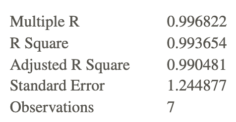
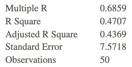
For 1-7, a lead English teacher is trying to determine the relationship between three tests given throughout the semester and the final exam. She decides to conduct a mini-study on this relationship and collects the test data (scores for Test 1, Test 2, Test 3, and the final exam) for 50 students in freshman English. She enters these data into Microsoft Excel and arrives at the following summary statistics:

ANOVA

	Df	SS	MS	F	Significance F
Regression	3	2342.7228	780.9076	13.621	0.0000
Residual	46	2637.2772	57.3321
Total	49	4980.0000

	Coefficients	Standard Error	t Stat	P-value
Intercept	10.7592	7.6268
Test 1	0.0506	0.1720	0.2941	0.7700
Test 2	0.5560	0.1431	3.885	0.0003
Test 3	0.2128	0.1782	1.194	0.2387

1. How many predictor variables are there in this scenario? What are the names of these predictor variables?
2. What does the regression coefficient for Test 2 tell us?
3. What is the regression model for this analysis?
4. What is the value of r₂, and what does it indicate?
5. Determine whether the multiple r-value is statistically significant.
6. Which of the predictor variables are statistically significant? What is the reasoning behind this decision?
7. Given this information, would you include all three predictor variables in the multiple regression model? Why or why not?

8. For all students at a particular university, the regression equation for y= college GPA and x1= high school GPA and x2 = college board score is ŷ =0.20+0.50x₁+0.002x₂
   a. Find the predicted college GPA for students
   • Having a high school GPA of 4.0 and college board score of 800.
   • x1=2.0,x2=200

   b. If a student retakes the college board exam and increases his score by 100 points, what will be the change in his predicted college GPA?

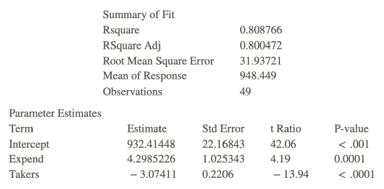
9. When, in 1982 SAT scores were first published on a state-by-state basis I the US there was a huge variation in the scores. This was positive for some states and a problem for other states. Some researchers wanted to study which certain variables were associated with the state SAT differences. The variable SAT is the average total SAT (verbal + quantitative) score in the state and the two explanatory variables they considered were Takers (the percent of total eligible students in a state who took the exam) and Expend (total state expenditure on secondary schools, expressed in hundreds of dollars per student). Following is a piece of computer output from this study:

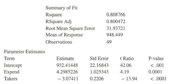
a. For Pennsylvania, SAT = 885, Takers = 50 and Expend = 27.98. What would you predict Pennsylvania’s average SAT score to be based on knowing its takers and expend, but not knowing its SAT? What is the residual for Pennsylvania

b. Use a test at the 0.05 significance level to test the hypothesis that Expend helps to predict SAT score once Takers are taken into account.

10. Below is some computer output of the regression of January Temperature vs Latitude and Longitude, where January Temperature is the dependent variable

Number of cases 57

RSquare = 74.1%

RSqAdj = 73.1%

X = 6.935 with 56 – 3 = 53 degrees of freedom

Variable	Coefficient	s.e. of Coeff	t-ratio	prob
Constant	98.6452	8.327	11.8	0.0001
Lat	−2.16355	0.1757	−12.3	0.0001
Long	0.133962	0.0631	2.12	0.0386

a. What is the regression equation?

b. What is the intercept and what does it represent?

c. For a fixed longitude, how does a change in latitude affect the January temperature?

d. Is there evidence that the longitude affects the January temperature for a given latitude? Test at the .05 level of significance.

11. Consider the following regression equation: ŷ =116.84+0.832x₁−0.951x₂+2.34x₃−1.08x4 Using the regression equation complete the following table for four different sets of specific values for explanatory variables:

Set	Weight (kg)	Age	Years	Pct_Life
	x1	x2	x3	x4	ŷ
1	65	30	15	50
2	65	50	15	30
3	65	50	25	50
4	65	50	35	70

12. Suppose that a college admissions committee plans to use data for total SAT score, high school grade point average and high school class rank to predict college freshman year grade point average for high school students applying for admission to the college. Write the regression model for this situation. Specify the response variable and the explanatory variables.
13. Describe an example of a multiple linear regression model for a topic that is of interest to you. Specify the response variable and the explanatory variables and write the multiple regression model for your example.
14. Suppose that a multiple linear regression model includes three explanatory variables.
    1. Write the population regression model using appropriate statistical notation.
    2. Explain the difference between what is represented by the symbol b₃ and the symbol β₃.

---

Review (Answers)

To view the Review answers, open this PDF file and look for section 9.4.

---

Vocabulary

Term	Definition
confidence intervals for regression coefficients	Confidence intervals for regression coefficients is the confidence level for multiple regression models.
multiple linear regression	In multiple linear regression, scores for the criterion variable are predicted using multiple predictor variables.
multiple regression coefficients	Multiple regression coefficients calculate the combined r^2 value and are done using a program such as Excel or SPSS.

---

Additional Resources

Video: Using Multiple Regression to Make a Prediction

Practice: Multiple Regression