
10.3: Inferences about Regression
- Page ID
- 5799
\( \newcommand{\vecs}[1]{\overset { \scriptstyle \rightharpoonup} {\mathbf{#1}} } \)
\( \newcommand{\vecd}[1]{\overset{-\!-\!\rightharpoonup}{\vphantom{a}\smash {#1}}} \)
\( \newcommand{\id}{\mathrm{id}}\) \( \newcommand{\Span}{\mathrm{span}}\)
( \newcommand{\kernel}{\mathrm{null}\,}\) \( \newcommand{\range}{\mathrm{range}\,}\)
\( \newcommand{\RealPart}{\mathrm{Re}}\) \( \newcommand{\ImaginaryPart}{\mathrm{Im}}\)
\( \newcommand{\Argument}{\mathrm{Arg}}\) \( \newcommand{\norm}[1]{\| #1 \|}\)
\( \newcommand{\inner}[2]{\langle #1, #2 \rangle}\)
\( \newcommand{\Span}{\mathrm{span}}\)
\( \newcommand{\id}{\mathrm{id}}\)
\( \newcommand{\Span}{\mathrm{span}}\)
\( \newcommand{\kernel}{\mathrm{null}\,}\)
\( \newcommand{\range}{\mathrm{range}\,}\)
\( \newcommand{\RealPart}{\mathrm{Re}}\)
\( \newcommand{\ImaginaryPart}{\mathrm{Im}}\)
\( \newcommand{\Argument}{\mathrm{Arg}}\)
\( \newcommand{\norm}[1]{\| #1 \|}\)
\( \newcommand{\inner}[2]{\langle #1, #2 \rangle}\)
\( \newcommand{\Span}{\mathrm{span}}\) \( \newcommand{\AA}{\unicode[.8,0]{x212B}}\)
\( \newcommand{\vectorA}[1]{\vec{#1}} % arrow\)
\( \newcommand{\vectorAt}[1]{\vec{\text{#1}}} % arrow\)
\( \newcommand{\vectorB}[1]{\overset { \scriptstyle \rightharpoonup} {\mathbf{#1}} } \)
\( \newcommand{\vectorC}[1]{\textbf{#1}} \)
\( \newcommand{\vectorD}[1]{\overrightarrow{#1}} \)
\( \newcommand{\vectorDt}[1]{\overrightarrow{\text{#1}}} \)
\( \newcommand{\vectE}[1]{\overset{-\!-\!\rightharpoonup}{\vphantom{a}\smash{\mathbf {#1}}}} \)
\( \newcommand{\vecs}[1]{\overset { \scriptstyle \rightharpoonup} {\mathbf{#1}} } \)
\( \newcommand{\vecd}[1]{\overset{-\!-\!\rightharpoonup}{\vphantom{a}\smash {#1}}} \)
\(\newcommand{\avec}{\mathbf a}\) \(\newcommand{\bvec}{\mathbf b}\) \(\newcommand{\cvec}{\mathbf c}\) \(\newcommand{\dvec}{\mathbf d}\) \(\newcommand{\dtil}{\widetilde{\mathbf d}}\) \(\newcommand{\evec}{\mathbf e}\) \(\newcommand{\fvec}{\mathbf f}\) \(\newcommand{\nvec}{\mathbf n}\) \(\newcommand{\pvec}{\mathbf p}\) \(\newcommand{\qvec}{\mathbf q}\) \(\newcommand{\svec}{\mathbf s}\) \(\newcommand{\tvec}{\mathbf t}\) \(\newcommand{\uvec}{\mathbf u}\) \(\newcommand{\vvec}{\mathbf v}\) \(\newcommand{\wvec}{\mathbf w}\) \(\newcommand{\xvec}{\mathbf x}\) \(\newcommand{\yvec}{\mathbf y}\) \(\newcommand{\zvec}{\mathbf z}\) \(\newcommand{\rvec}{\mathbf r}\) \(\newcommand{\mvec}{\mathbf m}\) \(\newcommand{\zerovec}{\mathbf 0}\) \(\newcommand{\onevec}{\mathbf 1}\) \(\newcommand{\real}{\mathbb R}\) \(\newcommand{\twovec}[2]{\left[\begin{array}{r}#1 \\ #2 \end{array}\right]}\) \(\newcommand{\ctwovec}[2]{\left[\begin{array}{c}#1 \\ #2 \end{array}\right]}\) \(\newcommand{\threevec}[3]{\left[\begin{array}{r}#1 \\ #2 \\ #3 \end{array}\right]}\) \(\newcommand{\cthreevec}[3]{\left[\begin{array}{c}#1 \\ #2 \\ #3 \end{array}\right]}\) \(\newcommand{\fourvec}[4]{\left[\begin{array}{r}#1 \\ #2 \\ #3 \\ #4 \end{array}\right]}\) \(\newcommand{\cfourvec}[4]{\left[\begin{array}{c}#1 \\ #2 \\ #3 \\ #4 \end{array}\right]}\) \(\newcommand{\fivevec}[5]{\left[\begin{array}{r}#1 \\ #2 \\ #3 \\ #4 \\ #5 \\ \end{array}\right]}\) \(\newcommand{\cfivevec}[5]{\left[\begin{array}{c}#1 \\ #2 \\ #3 \\ #4 \\ #5 \\ \end{array}\right]}\) \(\newcommand{\mattwo}[4]{\left[\begin{array}{rr}#1 \amp #2 \\ #3 \amp #4 \\ \end{array}\right]}\) \(\newcommand{\laspan}[1]{\text{Span}\{#1\}}\) \(\newcommand{\bcal}{\cal B}\) \(\newcommand{\ccal}{\cal C}\) \(\newcommand{\scal}{\cal S}\) \(\newcommand{\wcal}{\cal W}\) \(\newcommand{\ecal}{\cal E}\) \(\newcommand{\coords}[2]{\left\{#1\right\}_{#2}}\) \(\newcommand{\gray}[1]{\color{gray}{#1}}\) \(\newcommand{\lgray}[1]{\color{lightgray}{#1}}\) \(\newcommand{\rank}{\operatorname{rank}}\) \(\newcommand{\row}{\text{Row}}\) \(\newcommand{\col}{\text{Col}}\) \(\renewcommand{\row}{\text{Row}}\) \(\newcommand{\nul}{\text{Nul}}\) \(\newcommand{\var}{\text{Var}}\) \(\newcommand{\corr}{\text{corr}}\) \(\newcommand{\len}[1]{\left|#1\right|}\) \(\newcommand{\bbar}{\overline{\bvec}}\) \(\newcommand{\bhat}{\widehat{\bvec}}\) \(\newcommand{\bperp}{\bvec^\perp}\) \(\newcommand{\xhat}{\widehat{\xvec}}\) \(\newcommand{\vhat}{\widehat{\vvec}}\) \(\newcommand{\uhat}{\widehat{\uvec}}\) \(\newcommand{\what}{\widehat{\wvec}}\) \(\newcommand{\Sighat}{\widehat{\Sigma}}\) \(\newcommand{\lt}{<}\) \(\newcommand{\gt}{>}\) \(\newcommand{\amp}{&}\) \(\definecolor{fillinmathshade}{gray}{0.9}\)Inferences and Assumptions about Linear Regression
Hypothesis Testing for Linear Relationships
Let’s think for a minute about the relationship between correlation and the linear regression model. As we learned, if there is no correlation between the two variables X and Y, then it would be nearly impossible to fit a meaningful regression line to the points on a scatterplot graph. If there was no correlation, and our correlation value, or r-value, was 0, we would always come up with the same predicted value, which would be the mean of all the predicted values, or the mean of Ŷ . The figure below shows an example of what a regression line fit to variables with no correlation (r=0) would look like. As you can see, for any value of X, we always get the same predicted value of Y.
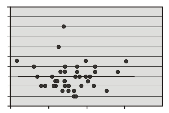
Using this knowledge, we can determine that if there is no relationship between X and Y, constructing a regression line doesn’t help us very much, because, again, the predicted score would always be the same. Therefore, when we estimate a linear regression model, we want to ensure that the regression coefficient, β, for the population does not equal zero. Furthermore, it is beneficial to test how strong (or far away) from zero the regression coefficient must be to strengthen our prediction of the Y scores.
In hypothesis testing of linear regression models, the null hypothesis to be tested is that the regression coefficient, β, equals zero. Our alternative hypothesis is that our regression coefficient does not equal zero.
H0: βHa: β=0≠0
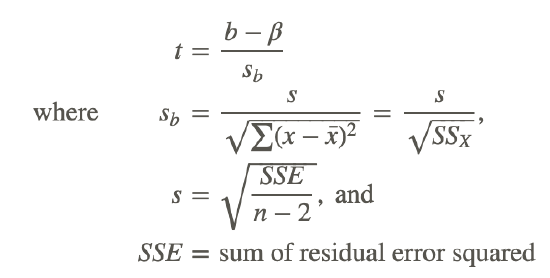
The test statistic for this hypothesis test is calculated as follows:
Testing the Accuracy of a Regression Equation
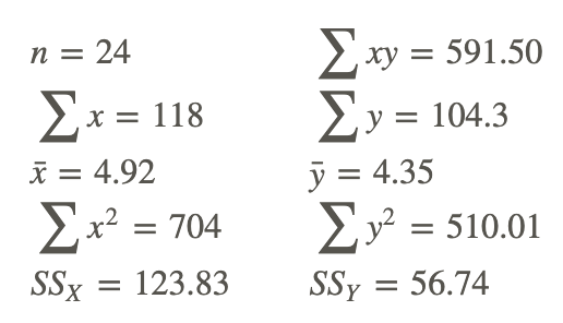
Let’s say that a football coach is using the results from a short physical fitness test to predict the results of a longer, more comprehensive one. He developed the regression equation Y=0.635X+1.22, and the standard error of estimate is 0.56. The summary statistics are as follows:
Summary statistics for two foot ball fitness tests.
Using α=0.05, test the null hypothesis that, in the population, the regression coefficient is zero, or H0: β=0.
We use the t-distribution to calculate the test statistic and find that the critical values in the t-distribution at 22 degrees of freedom are 2.074 standard scores above and below the mean. Also, the test statistic can be calculated as follows:
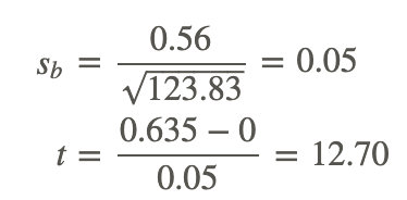
Since the observed value of the test statistic exceeds the critical value, the null hypothesis would be rejected, and we can conclude that if the null hypothesis were true, we would observe a regression coefficient of 0.635 by chance less than 5% of the time.
Making Inferences about Predicted Scores
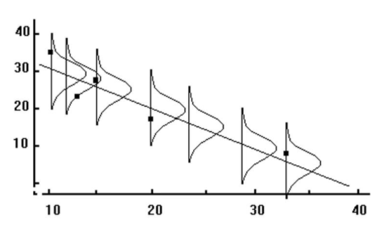
As we have mentioned, a regression line makes predictions about variables based on the relationship of the existing data. However, it is important to remember that the regression line simply infers, or estimates, what the value will be. These predictions are never accurate 100% of the time, unless there is a perfect correlation. What this means is that for every predicted value, we have a normal distribution (also known as the conditional distribution, since it is conditional on the X value) that describes the likelihood of obtaining other scores that are associated with the value of the predictor variable, X.
If we assume that these distributions are normal, we are able to make inferences about each of the predicted scores. We can ask questions like, “If the predictor variable, X, equals 4, what percentage of the distribution of Y scores will be lower than 3?”
The reason why we would ask questions like this depends on the scenario. Suppose, for example, that we want to know the percentage of students with a 5 on their short physical fitness test that have a predicted score higher than 5 on their long physical fitness test. If the coach is using this predicted score as a cutoff for playing in a varsity match, and this percentage is too low, he may want to consider changing the standards of the test.
To find the percentage of students with scores above or below a certain point, we use the concept of standard scores and the standard normal distribution.
Since we have a certain predicted value for every value of X, the Y values take on the shape of a normal distribution. This distribution has a mean (the regression line) and a standard error, which we found to be equal to 0.56. In short, the conditional distribution is used to determine the percentage of Y values above or below a certain value that are associated with a specific value of X.
Calculating Probability
Using our example above, if a student scored a 5 on the short test, what is the probability that he or she would have a score of 5 or greater on the long physical fitness test?
From the regression equation Y=0.635X+1.22, we find that the predicted score when the value of X is 5 is 4.40. Consider the conditional distribution of Y scores when the value of X is 5. Under our assumption, this distribution is normally distributed around the predicted value 4.40 and has a standard error of 0.56.
Therefore, to find the percentage of Y scores of 5 or greater, we use the general formula for a z-score to calculate the following:
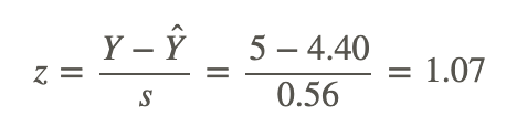
Using the z-distribution table, we find that the area to the right of a z-score of 1.07 is 0.1423. Therefore, we can conclude that the proportion of predicted scores of 5 or greater given a score of 5 on the short test is 0.1423, or 14.23%.
Prediction Intervals
Similar to hypothesis testing for samples and populations, we can also build a confidence interval around our regression results. This helps us ask questions like “If the predictor variable, X, is equal to a certain value, what are the likely values for Y?” A confidence interval gives us a range of scores that has a certain percent probability of including the score that we are after.
We know that the standard error of the predicted score is smaller when the predicted value is close to the actual value, and it increases as X deviates from the mean. This means that the weaker of a predictor that the regression line is, the larger the standard error of the predicted score will be. The formulas for the standard error of a predicted score and a confidence interval are as follows:
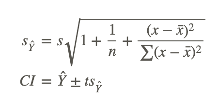
where:
Ŷ is the predicted score.
t is the critical value for n−2 degrees of freedom.
sŶ is the standard error of the predicted score.
Developing Confidence Intervals
Develop a 95% confidence interval for the predicted score of a student who scores a 4 on the short physical fitness exam.
We calculate the standard error of the predicted score using the formula as follows:

Using the general formula for a confidence interval, we can calculate the answer as shown:
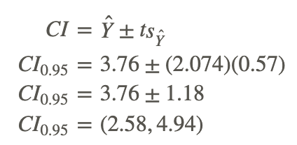
Therefore, we can say that we are 95% confident that given a student's short physical fitness test score, X, of 4, the interval from 2.58 to 4.94 will contain the student's score for the longer physical fitness test.
Regression Assumptions
We make several assumptions under a linear regression model, including:
At each value of X, there is a distribution of Y. These distributions have a mean centered at the predicted value and a standard error that is calculated using the sum of squares.
Using a regression model to predict scores only works if the regression line is a good fit to the data. If this relationship is non-linear, we could either transform the data (i.e., a logarithmic transformation) or try one of the other regression equations that are available with Excel or a graphing calculator.
The standard deviations and the variances of each of these distributions for each of the predicted values are equal. This is called homoscedasticity.
Finally, for each given value of X, the values of Y are independent of each other.
Example
The following example uses data from the previous section:
Verbal SAT scores were used to predict the GPA of students. From the data, we found this least squares regression line:
Ŷ =0.0055X+0.097
We also found that SSE=0.26 for the n=7 samples.
Example 1
Suppose a student scores a 650 on the verbal SAT. Assuming the data is normally distributed, what is the probability that they will have a GPA of at least 3.8?
Using the least squares regression line, we will predict the GPA for a verbal SAT score of 650:
Ŷ =0.0055(650)+0.097=3.575+0.097=3.672
This means that an SAT score of 650 predicts that the student will have a GPA of 3.672. They could have a higher, or a lower GPA though, so now we will look at the probability that a student with a GRE score of 650 has a GPA of at least 3.8. First we have to find:
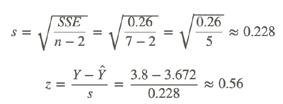
Now we simply look at the z-table to find the probability of getting a z-score of 0.56 or higher.
P(z>0.56)=0.288.
The probability of having a GPA of at least 3.8 when scoring a 650 on the verbal SAT is 0.288.
Review
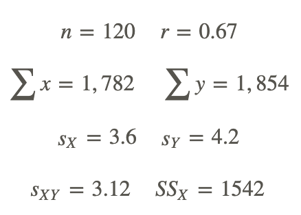
For 1-10, a college counselor is putting on a presentation about the financial benefits of further education and takes a random sample of 120 parents. Each parent was asked a number of questions, including the number of years of education that he or she has (including college) and his or her yearly income (recorded in the thousands of dollars). The summary data for this survey are as follows:
- this decision?
- Do you think that these two variables (income and level of formal education) are correlated? Is so, please describe the nature of their relationship.
- What would be the regression equation for predicting income, Y, from the level of education, X?
- Using this regression equation, predict the income for a person with 2 years of college (13.5 years of formal education).
- Test the null hypothesis that in the population, the regression coefficient for this scenario is zero.
- First develop the null and alternative hypotheses.
- Set the critical value to α=0.05.
- Compute the test statistic.
- Make a decision regarding the null hypothesis.
- For those parents with 15 years of formal education, what is the percentage who will have an annual income greater than $18,500?
- For those parents with 12 years of formal education, what is the percentage who will have an annual income greater than $18,500?
- Develop a 95% confidence interval for the predicted annual income when a parent indicates that he or she has a college degree (i.e., 16 years of formal education).
- If you were the college counselor, what would you say in the presentation to the parents and students about the relationship between further education and salary? Would you encourage students to further their education based on these analyses? Why or why not?
- Using the same null and alternative hypotheses, and test statistics as you did in question 5, make a decision at the significance level of α=0.01.
Vocabulary
| Term | Definition |
|---|---|
| homoscedasticity | Homoscedasticity occurs when the standard deviations and the variances of each of these distributions for each of the predicted values are equal. |
| linear regression model | When we estimate a linear regression model, we want to ensure that the regression coefficient for the population, beta, does not equal zero. |
| predicted values | The positive predictive value is the probability that a test gives a true result for a true statistic. The negative predictive value is the probability that a test gives a false result for a false statistic |
| predictor variable | A predictor variable is a variable that can be used to predict the value of another variable (as in statistical regression). |
| regression coefficient | The regression coefficient (or the slope) explains the nature of the relationship between the two variables. |