2.7.6: Graph Inverse Trigonometric Functions
- Page ID
- 14942
\( \newcommand{\vecs}[1]{\overset { \scriptstyle \rightharpoonup} {\mathbf{#1}} } \)
\( \newcommand{\vecd}[1]{\overset{-\!-\!\rightharpoonup}{\vphantom{a}\smash {#1}}} \)
\( \newcommand{\id}{\mathrm{id}}\) \( \newcommand{\Span}{\mathrm{span}}\)
( \newcommand{\kernel}{\mathrm{null}\,}\) \( \newcommand{\range}{\mathrm{range}\,}\)
\( \newcommand{\RealPart}{\mathrm{Re}}\) \( \newcommand{\ImaginaryPart}{\mathrm{Im}}\)
\( \newcommand{\Argument}{\mathrm{Arg}}\) \( \newcommand{\norm}[1]{\| #1 \|}\)
\( \newcommand{\inner}[2]{\langle #1, #2 \rangle}\)
\( \newcommand{\Span}{\mathrm{span}}\)
\( \newcommand{\id}{\mathrm{id}}\)
\( \newcommand{\Span}{\mathrm{span}}\)
\( \newcommand{\kernel}{\mathrm{null}\,}\)
\( \newcommand{\range}{\mathrm{range}\,}\)
\( \newcommand{\RealPart}{\mathrm{Re}}\)
\( \newcommand{\ImaginaryPart}{\mathrm{Im}}\)
\( \newcommand{\Argument}{\mathrm{Arg}}\)
\( \newcommand{\norm}[1]{\| #1 \|}\)
\( \newcommand{\inner}[2]{\langle #1, #2 \rangle}\)
\( \newcommand{\Span}{\mathrm{span}}\) \( \newcommand{\AA}{\unicode[.8,0]{x212B}}\)
\( \newcommand{\vectorA}[1]{\vec{#1}} % arrow\)
\( \newcommand{\vectorAt}[1]{\vec{\text{#1}}} % arrow\)
\( \newcommand{\vectorB}[1]{\overset { \scriptstyle \rightharpoonup} {\mathbf{#1}} } \)
\( \newcommand{\vectorC}[1]{\textbf{#1}} \)
\( \newcommand{\vectorD}[1]{\overrightarrow{#1}} \)
\( \newcommand{\vectorDt}[1]{\overrightarrow{\text{#1}}} \)
\( \newcommand{\vectE}[1]{\overset{-\!-\!\rightharpoonup}{\vphantom{a}\smash{\mathbf {#1}}}} \)
\( \newcommand{\vecs}[1]{\overset { \scriptstyle \rightharpoonup} {\mathbf{#1}} } \)
\( \newcommand{\vecd}[1]{\overset{-\!-\!\rightharpoonup}{\vphantom{a}\smash {#1}}} \)
\(\newcommand{\avec}{\mathbf a}\) \(\newcommand{\bvec}{\mathbf b}\) \(\newcommand{\cvec}{\mathbf c}\) \(\newcommand{\dvec}{\mathbf d}\) \(\newcommand{\dtil}{\widetilde{\mathbf d}}\) \(\newcommand{\evec}{\mathbf e}\) \(\newcommand{\fvec}{\mathbf f}\) \(\newcommand{\nvec}{\mathbf n}\) \(\newcommand{\pvec}{\mathbf p}\) \(\newcommand{\qvec}{\mathbf q}\) \(\newcommand{\svec}{\mathbf s}\) \(\newcommand{\tvec}{\mathbf t}\) \(\newcommand{\uvec}{\mathbf u}\) \(\newcommand{\vvec}{\mathbf v}\) \(\newcommand{\wvec}{\mathbf w}\) \(\newcommand{\xvec}{\mathbf x}\) \(\newcommand{\yvec}{\mathbf y}\) \(\newcommand{\zvec}{\mathbf z}\) \(\newcommand{\rvec}{\mathbf r}\) \(\newcommand{\mvec}{\mathbf m}\) \(\newcommand{\zerovec}{\mathbf 0}\) \(\newcommand{\onevec}{\mathbf 1}\) \(\newcommand{\real}{\mathbb R}\) \(\newcommand{\twovec}[2]{\left[\begin{array}{r}#1 \\ #2 \end{array}\right]}\) \(\newcommand{\ctwovec}[2]{\left[\begin{array}{c}#1 \\ #2 \end{array}\right]}\) \(\newcommand{\threevec}[3]{\left[\begin{array}{r}#1 \\ #2 \\ #3 \end{array}\right]}\) \(\newcommand{\cthreevec}[3]{\left[\begin{array}{c}#1 \\ #2 \\ #3 \end{array}\right]}\) \(\newcommand{\fourvec}[4]{\left[\begin{array}{r}#1 \\ #2 \\ #3 \\ #4 \end{array}\right]}\) \(\newcommand{\cfourvec}[4]{\left[\begin{array}{c}#1 \\ #2 \\ #3 \\ #4 \end{array}\right]}\) \(\newcommand{\fivevec}[5]{\left[\begin{array}{r}#1 \\ #2 \\ #3 \\ #4 \\ #5 \\ \end{array}\right]}\) \(\newcommand{\cfivevec}[5]{\left[\begin{array}{c}#1 \\ #2 \\ #3 \\ #4 \\ #5 \\ \end{array}\right]}\) \(\newcommand{\mattwo}[4]{\left[\begin{array}{rr}#1 \amp #2 \\ #3 \amp #4 \\ \end{array}\right]}\) \(\newcommand{\laspan}[1]{\text{Span}\{#1\}}\) \(\newcommand{\bcal}{\cal B}\) \(\newcommand{\ccal}{\cal C}\) \(\newcommand{\scal}{\cal S}\) \(\newcommand{\wcal}{\cal W}\) \(\newcommand{\ecal}{\cal E}\) \(\newcommand{\coords}[2]{\left\{#1\right\}_{#2}}\) \(\newcommand{\gray}[1]{\color{gray}{#1}}\) \(\newcommand{\lgray}[1]{\color{lightgray}{#1}}\) \(\newcommand{\rank}{\operatorname{rank}}\) \(\newcommand{\row}{\text{Row}}\) \(\newcommand{\col}{\text{Col}}\) \(\renewcommand{\row}{\text{Row}}\) \(\newcommand{\nul}{\text{Nul}}\) \(\newcommand{\var}{\text{Var}}\) \(\newcommand{\corr}{\text{corr}}\) \(\newcommand{\len}[1]{\left|#1\right|}\) \(\newcommand{\bbar}{\overline{\bvec}}\) \(\newcommand{\bhat}{\widehat{\bvec}}\) \(\newcommand{\bperp}{\bvec^\perp}\) \(\newcommand{\xhat}{\widehat{\xvec}}\) \(\newcommand{\vhat}{\widehat{\vvec}}\) \(\newcommand{\uhat}{\widehat{\uvec}}\) \(\newcommand{\what}{\widehat{\wvec}}\) \(\newcommand{\Sighat}{\widehat{\Sigma}}\) \(\newcommand{\lt}{<}\) \(\newcommand{\gt}{>}\) \(\newcommand{\amp}{&}\) \(\definecolor{fillinmathshade}{gray}{0.9}\)Domain and range of inverse functions.
In order for inverses of functions to be functions, the original function must pass the horizontal line test. Though none of the trigonometric functions pass the horizontal line test, you can restrict their domains so that they can pass. Then the inverses are produced just like with normal functions. Once you have the basic inverse functions, the normal transformation rules apply.
Why is \(\sin^{-1}\left(\sin 370^{\circ}\right)\neq 370^{\circ}\)? Don’t the arcsin and sin just cancel out?
Graphs of Inverse Trigonometric Functions
Since none of the six trigonometric functions pass the horizontal line test, you must restrict their domains before finding inverses of these functions. This is just like the way \(y=\sqrt{x}\) is the inverse of \(y=x^2\) when you restrict the domain to \(x\geq 0\).
Consider the sine graph:
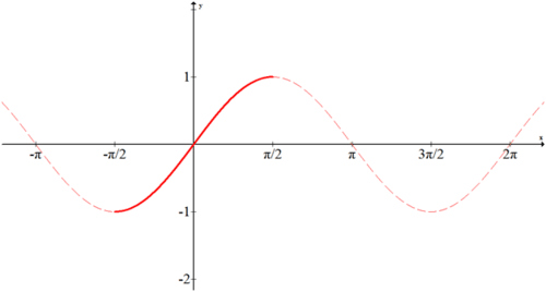
As a general rule, the restrictions to the domain are either the interval \(\left[−\dfrac{\pi}{2},\dfrac{\pi}{2}\right]\) or \([0,\pi ]\) to keep things simple. In this case sine is restricted to \(\left[−\dfrac{\pi}{2},\dfrac{\pi}{2}\right]\), as shown above. To find the inverse, reflect the bold portion across the line \(y=x\). The blue curve below shows \(f(x)=\sin^{-1}x\).
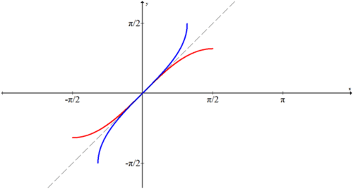
The result of this inversion is that arcsine will only ever produce angles between \(−\dfrac{\pi}{2}\) and \(\dfrac{\pi}{2}\).
The blue curve below shows \(f(x)=\cos^{-1} x\)?
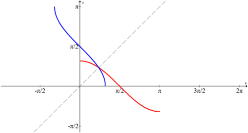
The portion of cosine that fits the horizontal line test is the interval \([0, \pi ]\). To find the inverse, that portion is reflected across the line \(y=x\).
Earlier, you were asked why sine and arcsine don't always just cancel out.
Solution
Since arcsine only produces angles between \(−\dfrac{\pi}{2}\) and \(\dfrac{\pi}{2}\) or \(−90^{\circ}\) to \(+90^{\circ}\) the result of \(\sin^{-1}(\sin 370^{\circ})\) is \(10^{\circ}\) which is coterminal to \(370^{\circ}\).
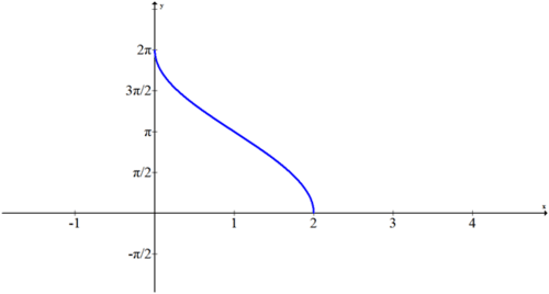
Graph the function \(f(x)=2\cos^{-1}(x−1)\).
Solution
Since \(f(x)=\cos^{-1}x\) was graphed earlier, now you just need to shift it right one unit and stretch it vertically by a factor of 2. It intersected the x axis at 1 before and now it will intersect at 2. It reached a height of \(\pi \) before and now it will reach a height of \(2\pi \).
Evaluate the following expression with and without a calculator using right triangles and your knowledge of inverse trigonometric functions.
\(\cot\left(\csc^{-1}\left(-\dfrac{13}{5}\right)\right)\)
Solution
In order to be able to effectively calculate this out it is best to write the expression explicitly only in terms of functions that your calculator does have. Be aware that some calculators have both \(\sin^{-1}x\) and \((\sin x)^{−1}\).
The hardest part of this question is seeing the csc as a function (which produces an angle) on a ratio of a hypotenuse of 13 and an opposite side of -5. The sine of the inverse ratio must produce the same angle, so you can substitute it.
- \(\csc^{-1}\left(-\dfrac{13}{5}\right)=\sin^{-1}(−\dfrac{5}{13})\)
- \(\cot(\theta )=\dfrac{1}{\tan\theta}\)
\(\cot\left(\csc^{-1}\left(-\dfrac{13}{5}\right)\right)=\dfrac{1}{\tan \left(\sin^{-1}\left(−\dfrac{5}{13}\right)\right)}=−\dfrac{12}{5}\)
Start with your knowledge that \(\csc^{-1}\left(-\dfrac{13}{5}\right)\) describes an angle in the third or the fourth quadrant because those are the two quadrants where cosecant is negative. Since \(\csc^{-1}\theta \) has range \(−\dfrac{\pi}{2},\dfrac{\pi}{2}\), it only produces angles in quadrant I or quadrant IV. This triangle must then be in the fourth quadrant. All you need to do is draw the triangle and identify the cotangent ratio.
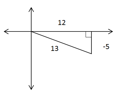
Cotangent is adjacent over opposite.
\(\cot\left(\csc^{-1}\left(−\dfrac{13}{5}\right)\right)=−\dfrac{12}{5}\)
What is the graph of \(y=\tan^{-1}x\)?
Solution
Graph the portion of tangent that fits the horizontal line test and reflect across the line y=x. Note that the graph of arctan is in blue.

What is the graph of \(y=\csc^{-1}x\)
Solution
Graph the portion of cosecant that fits the horizontal line test and reflect across the line y=x.
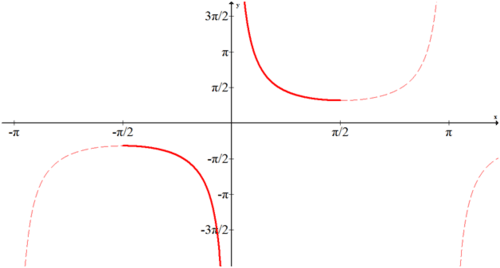
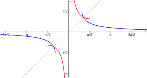
Note that \(f(x)=\csc^{-1}x\) is in blue.
Review
- Graph \(f(x)=\cot^{-1}x\).
- Graph \(g(x)=\sec^{-1}x\).
Name each of the following graphs.
-
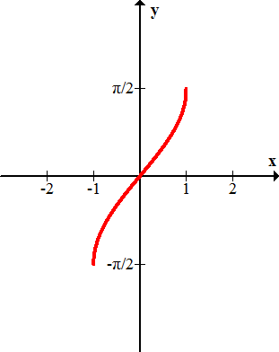
Figure \(\PageIndex{8}\) -
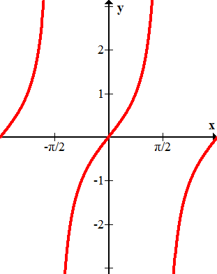
Figure \(\PageIndex{9}\) -
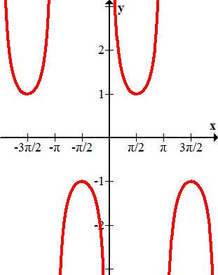
Figure \(\PageIndex{10}\) -
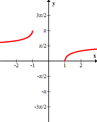
Figure \(\PageIndex{11}\) -
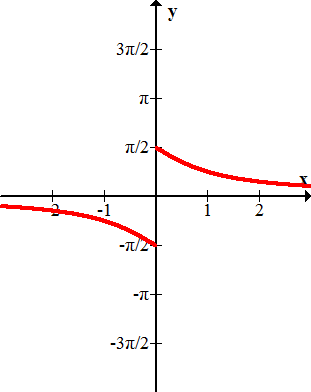
Figure \(\PageIndex{12}\)
Graph each of the following functions using your knowledge of function transformations.
- \(h(x)=3\sin^{-1}(x+1)\)
- \(k(x)=2\sin^{-1}(x)+\dfrac{\pi}{2}\)
- \(m(x)=−\cos^{-1}(x−2)\)
- \(j(x)=\cot^{-1}(x)+\pi\)
- \(p(x)=−2\tan^{-1}(x−1)\)
- \(q(x)=\csc^{-1}(x−2)\)
- \(r(x)=−\sec^{-1}(x)+4\)
- \(t(x)=\csc^{-1}(x+1)−\dfrac{3 \pi}{2}\)
- \(v(x)=2\sec^{-1}(x+2)+\dfrac{\pi}{2}\)
- \(w(x)=−\cot^{-1}(x)−\dfrac{\pi}{2}\)
Evaluate each expression.
- \(\sec \left(\tan^{-1}\left[\dfrac{3}{4}\right]\right)\)
- \(\cot \left(\csc^{-1} \left[\dfrac{13}{12}\right]\right)\)
- \(\csc \left(\tan^{-1} \left[\dfrac{4}{3}\right]\right)\)
Review (Answers)
To see the Review answers, open this PDF file and look for section 5.8.
Vocabulary
| Term | Definition |
|---|---|
| Cosecant | The cosecant of an angle in a right triangle is a relationship found by dividing the length of the hypotenuse by the length of the side opposite to the given angle. This is the reciprocal of the sine function. |
| Cotangent | The cotangent of an angle in a right triangle is a relationship found by dividing the length of the side adjacent to the given angle by the length of the side opposite to the given angle. This is the reciprocal of the tangent function. |
| Coterminal | Two angles are coterminal if they are drawn in the standard position and both have terminal sides that are at the same location. |
| domain | The domain of a function is the set of x-values for which the function is defined. |
| Horizontal Line Test | The horizontal line test says that if a horizontal line drawn anywhere through the graph of a function intersects the function in more than one location, then the function is not one-to-one and not invertible. |
| restricted domain | Restricted domain refers to the fact that when creating an inverse you sometimes must cut off the domain of most of the function, saving the largest possible portion so that when the inverse is created it is also a function. |
| Secant | The secant of an angle in a right triangle is the value found by dividing length of the hypotenuse by the length of the side adjacent the given angle. The secant ratio is the reciprocal of the cosine ratio. |
| Transformations | Transformations are used to change the graph of a parent function into the graph of a more complex function. |
Additional Resources
Practice: Graph Inverse Trigonometric Functions

