2.7.5: Cosine and Secant Graphs
- Page ID
- 14941
\( \newcommand{\vecs}[1]{\overset { \scriptstyle \rightharpoonup} {\mathbf{#1}} } \)
\( \newcommand{\vecd}[1]{\overset{-\!-\!\rightharpoonup}{\vphantom{a}\smash {#1}}} \)
\( \newcommand{\id}{\mathrm{id}}\) \( \newcommand{\Span}{\mathrm{span}}\)
( \newcommand{\kernel}{\mathrm{null}\,}\) \( \newcommand{\range}{\mathrm{range}\,}\)
\( \newcommand{\RealPart}{\mathrm{Re}}\) \( \newcommand{\ImaginaryPart}{\mathrm{Im}}\)
\( \newcommand{\Argument}{\mathrm{Arg}}\) \( \newcommand{\norm}[1]{\| #1 \|}\)
\( \newcommand{\inner}[2]{\langle #1, #2 \rangle}\)
\( \newcommand{\Span}{\mathrm{span}}\)
\( \newcommand{\id}{\mathrm{id}}\)
\( \newcommand{\Span}{\mathrm{span}}\)
\( \newcommand{\kernel}{\mathrm{null}\,}\)
\( \newcommand{\range}{\mathrm{range}\,}\)
\( \newcommand{\RealPart}{\mathrm{Re}}\)
\( \newcommand{\ImaginaryPart}{\mathrm{Im}}\)
\( \newcommand{\Argument}{\mathrm{Arg}}\)
\( \newcommand{\norm}[1]{\| #1 \|}\)
\( \newcommand{\inner}[2]{\langle #1, #2 \rangle}\)
\( \newcommand{\Span}{\mathrm{span}}\) \( \newcommand{\AA}{\unicode[.8,0]{x212B}}\)
\( \newcommand{\vectorA}[1]{\vec{#1}} % arrow\)
\( \newcommand{\vectorAt}[1]{\vec{\text{#1}}} % arrow\)
\( \newcommand{\vectorB}[1]{\overset { \scriptstyle \rightharpoonup} {\mathbf{#1}} } \)
\( \newcommand{\vectorC}[1]{\textbf{#1}} \)
\( \newcommand{\vectorD}[1]{\overrightarrow{#1}} \)
\( \newcommand{\vectorDt}[1]{\overrightarrow{\text{#1}}} \)
\( \newcommand{\vectE}[1]{\overset{-\!-\!\rightharpoonup}{\vphantom{a}\smash{\mathbf {#1}}}} \)
\( \newcommand{\vecs}[1]{\overset { \scriptstyle \rightharpoonup} {\mathbf{#1}} } \)
\( \newcommand{\vecd}[1]{\overset{-\!-\!\rightharpoonup}{\vphantom{a}\smash {#1}}} \)
\(\newcommand{\avec}{\mathbf a}\) \(\newcommand{\bvec}{\mathbf b}\) \(\newcommand{\cvec}{\mathbf c}\) \(\newcommand{\dvec}{\mathbf d}\) \(\newcommand{\dtil}{\widetilde{\mathbf d}}\) \(\newcommand{\evec}{\mathbf e}\) \(\newcommand{\fvec}{\mathbf f}\) \(\newcommand{\nvec}{\mathbf n}\) \(\newcommand{\pvec}{\mathbf p}\) \(\newcommand{\qvec}{\mathbf q}\) \(\newcommand{\svec}{\mathbf s}\) \(\newcommand{\tvec}{\mathbf t}\) \(\newcommand{\uvec}{\mathbf u}\) \(\newcommand{\vvec}{\mathbf v}\) \(\newcommand{\wvec}{\mathbf w}\) \(\newcommand{\xvec}{\mathbf x}\) \(\newcommand{\yvec}{\mathbf y}\) \(\newcommand{\zvec}{\mathbf z}\) \(\newcommand{\rvec}{\mathbf r}\) \(\newcommand{\mvec}{\mathbf m}\) \(\newcommand{\zerovec}{\mathbf 0}\) \(\newcommand{\onevec}{\mathbf 1}\) \(\newcommand{\real}{\mathbb R}\) \(\newcommand{\twovec}[2]{\left[\begin{array}{r}#1 \\ #2 \end{array}\right]}\) \(\newcommand{\ctwovec}[2]{\left[\begin{array}{c}#1 \\ #2 \end{array}\right]}\) \(\newcommand{\threevec}[3]{\left[\begin{array}{r}#1 \\ #2 \\ #3 \end{array}\right]}\) \(\newcommand{\cthreevec}[3]{\left[\begin{array}{c}#1 \\ #2 \\ #3 \end{array}\right]}\) \(\newcommand{\fourvec}[4]{\left[\begin{array}{r}#1 \\ #2 \\ #3 \\ #4 \end{array}\right]}\) \(\newcommand{\cfourvec}[4]{\left[\begin{array}{c}#1 \\ #2 \\ #3 \\ #4 \end{array}\right]}\) \(\newcommand{\fivevec}[5]{\left[\begin{array}{r}#1 \\ #2 \\ #3 \\ #4 \\ #5 \\ \end{array}\right]}\) \(\newcommand{\cfivevec}[5]{\left[\begin{array}{c}#1 \\ #2 \\ #3 \\ #4 \\ #5 \\ \end{array}\right]}\) \(\newcommand{\mattwo}[4]{\left[\begin{array}{rr}#1 \amp #2 \\ #3 \amp #4 \\ \end{array}\right]}\) \(\newcommand{\laspan}[1]{\text{Span}\{#1\}}\) \(\newcommand{\bcal}{\cal B}\) \(\newcommand{\ccal}{\cal C}\) \(\newcommand{\scal}{\cal S}\) \(\newcommand{\wcal}{\cal W}\) \(\newcommand{\ecal}{\cal E}\) \(\newcommand{\coords}[2]{\left\{#1\right\}_{#2}}\) \(\newcommand{\gray}[1]{\color{gray}{#1}}\) \(\newcommand{\lgray}[1]{\color{lightgray}{#1}}\) \(\newcommand{\rank}{\operatorname{rank}}\) \(\newcommand{\row}{\text{Row}}\) \(\newcommand{\col}{\text{Col}}\) \(\renewcommand{\row}{\text{Row}}\) \(\newcommand{\nul}{\text{Nul}}\) \(\newcommand{\var}{\text{Var}}\) \(\newcommand{\corr}{\text{corr}}\) \(\newcommand{\len}[1]{\left|#1\right|}\) \(\newcommand{\bbar}{\overline{\bvec}}\) \(\newcommand{\bhat}{\widehat{\bvec}}\) \(\newcommand{\bperp}{\bvec^\perp}\) \(\newcommand{\xhat}{\widehat{\xvec}}\) \(\newcommand{\vhat}{\widehat{\vvec}}\) \(\newcommand{\uhat}{\widehat{\uvec}}\) \(\newcommand{\what}{\widehat{\wvec}}\) \(\newcommand{\Sighat}{\widehat{\Sigma}}\) \(\newcommand{\lt}{<}\) \(\newcommand{\gt}{>}\) \(\newcommand{\amp}{&}\) \(\definecolor{fillinmathshade}{gray}{0.9}\)Wave based on x value and radius of a circle; graph based on the reciprocal.
Imagine for a moment that you have a clock that has only one hand - that rotates counterclockwise!. However, the hand is very slim all the way until the tip, where there is a ball on the end. In fact, the hand is so slim you won't notice it. You only notice the ball on the end of the rotating hand. This hand is rotating faster than normal.

Consider what it would be like if you put a light above the clock and let the shadow of the hands fall on the wall under the clock. What pattern would that shadow trace out? If you think about it, you might realize that the shadow would make an left and right motion, over and over as the hand of the clock rotated. Now imagine that instead of a wall, there was a large piece of paper for the shadow to fall on. And wherever the shadow fell, there would be a mark on the paper. Finally, imagine moving the paper as the clock rotates. Can you imagine sort of pattern this would trace out?
Cosine and Secant Graphs
If you have read other Trigonometry sections in this course, you may have learned that sine and cosine are very closely related. The cosine of an angle is the same as the sine of its complementary angle. So, it should not be a surprise that sine and cosine waves are very similar in that they are both periodic with a period of \(2\pi \), a range from -1 to 1, and a domain of all real angles.
The cosine of an angle is the ratio of \(\dfrac{x}{r}\), so in the unit circle, the cosine is the x−coordinate of the point of rotation. If we trace the x−coordinate through a rotation, notice the change in the distance of \(\cos x\) starts at one. The x−coordinate at \(0^{\circ}\) is 1 and the x−coordinate for \(90^{\circ}\) is 0, so the cosine value is decreasing from 1 to 0 through the 1st quadrant.
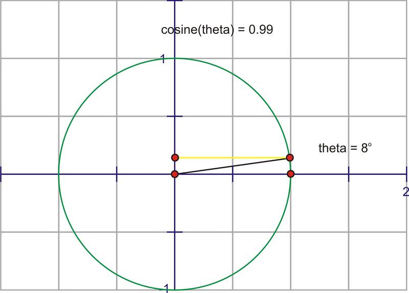
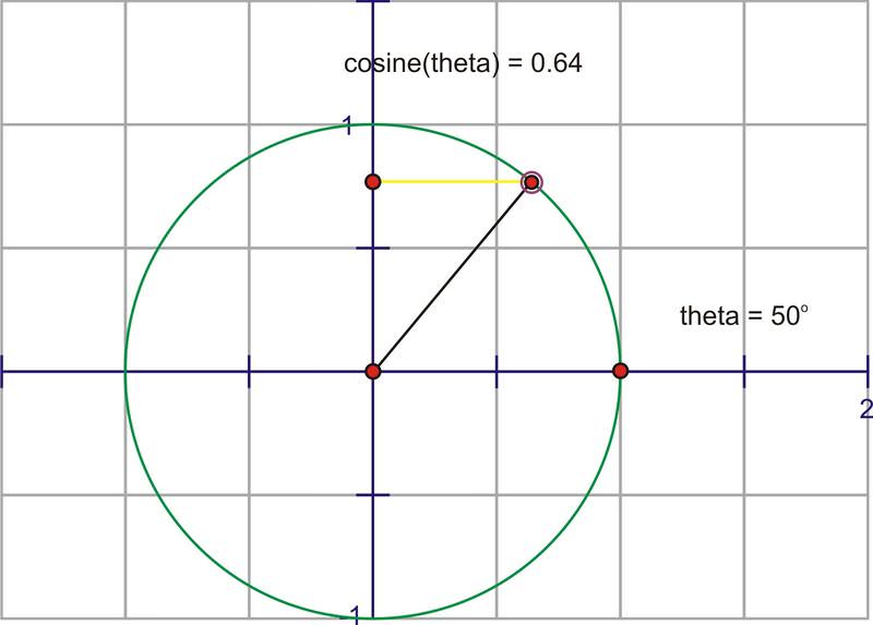
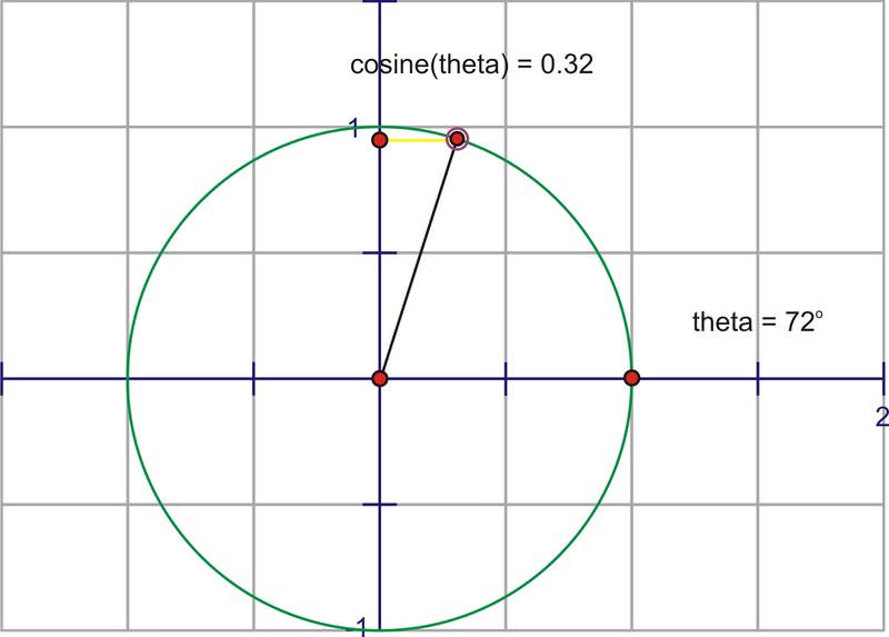
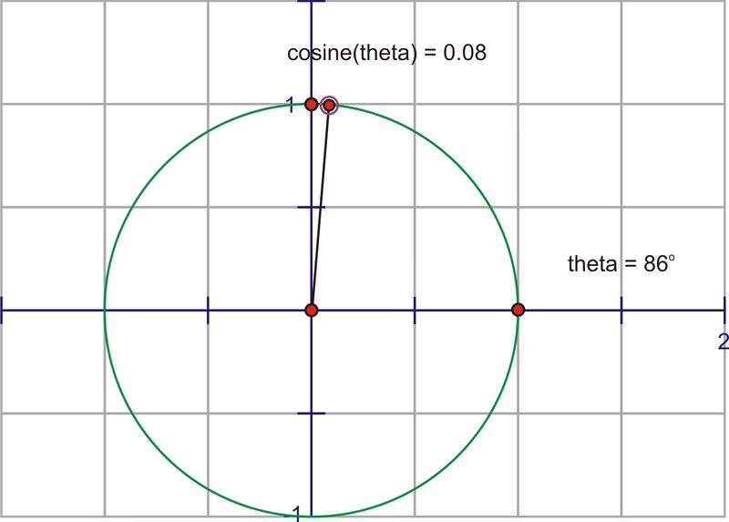
Here is a sequence of rotations. Compare the x− coordinate of the point of rotation with the height of the point as it traces along the horizontal. These pictures plot \((\theta ,\cos \theta )\) on the coordinate plane as \((x,y)\).


Plotting the quadrant angles and filling in the in-between values shows the graph of \(y=\cos x\)
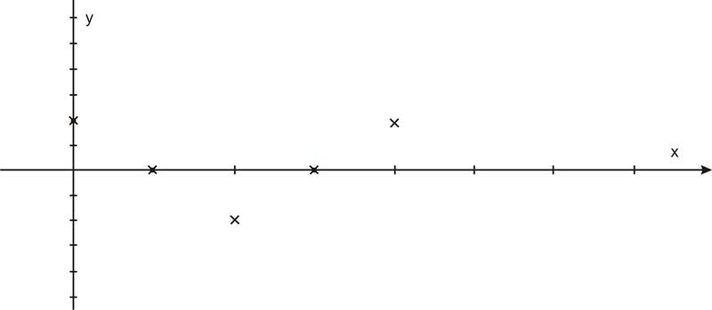

The graph of \(y=\cos x\) has a period of \(2\pi \). The range of a cosine curve is \({−1\leq y\leq 1}\) and the domain of \(\cos x\) is all reals. If you've studied the sine function, you may notice that the shape of the curve is exactly the same, but shifted by \(\dfrac{\pi }{2}\).
Secant is the reciprocal of cosine, or \(\dfrac{1}{x}\). Therefore, whenever the cosine is zero, the secant is going to have a vertical asymptote because it will be undefined. It also has the same sign as the cosine function in the same quadrants. Here is the graph.
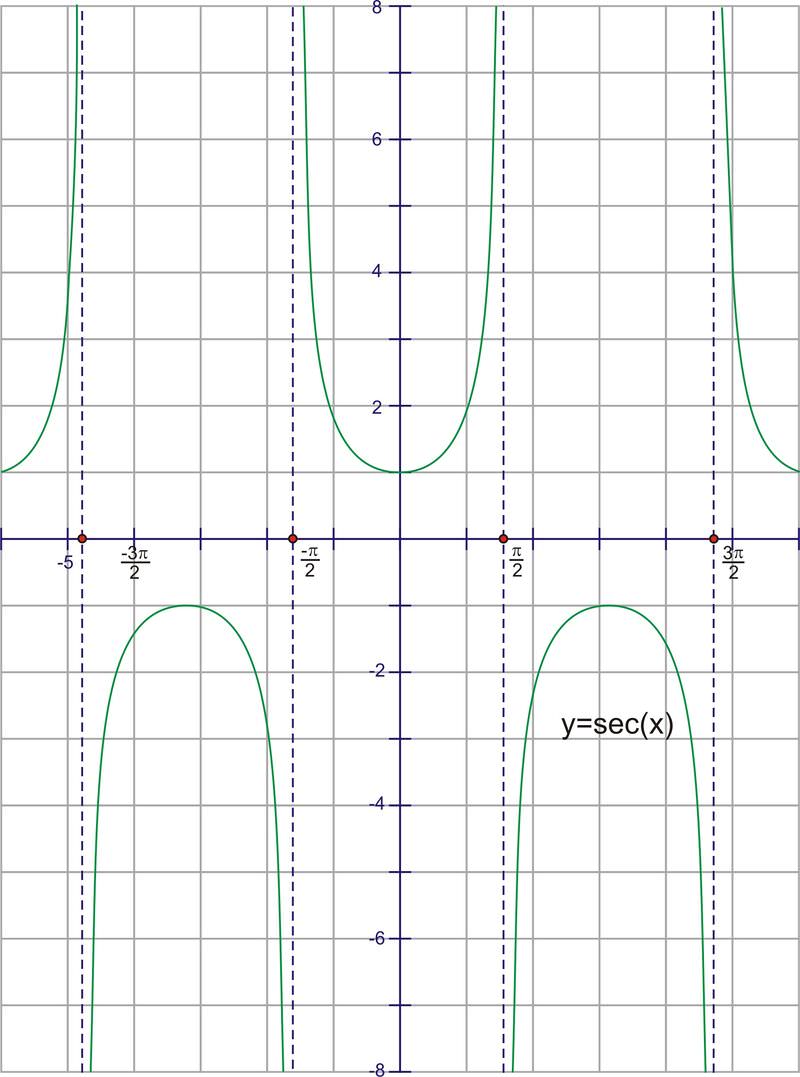
The period of the function is \(2\pi \), just like cosine. The domain of the function is all real numbers, except multiples of \(\pi \) starting at \(\dfrac{\pi }{2} \cdot \left\{\ldots, −\dfrac{\pi }{2},\dfrac{\pi }{2}, 0, \dfrac{3\pi }{2}, \dfrac{5 \pi }{2} \ldots \right\}\). The range is all real numbers greater than or equal to 1 as well as all real numbers less than or equal to -1. Notice that the range is everything except where cosine is defined (other than the tops and bottoms of the cosine curve).
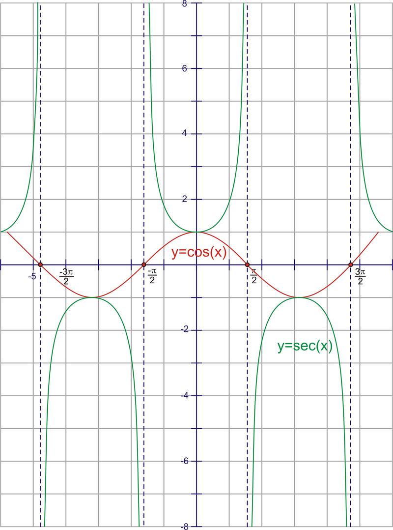
Notice again the reciprocal relationships at 0 and the asymptotes. Also look at the intersection points of the graphs at 1 and -1. Again, this graph looks parabolic, but it is not.
Sketch the graph
Sketch a graph of \(h(x)=5+\dfrac{1}{2}\sec 4x\) over the interval \([0,2\pi ]\).
If you compare this example to \(f(x)=\sec x\), it will be translated 5 units up, with an amplitude of \(\dfrac{1}{2}\) and a frequency of 4. This means in our interval of 0 to \(2\pi \), there will be 4 secant curves.
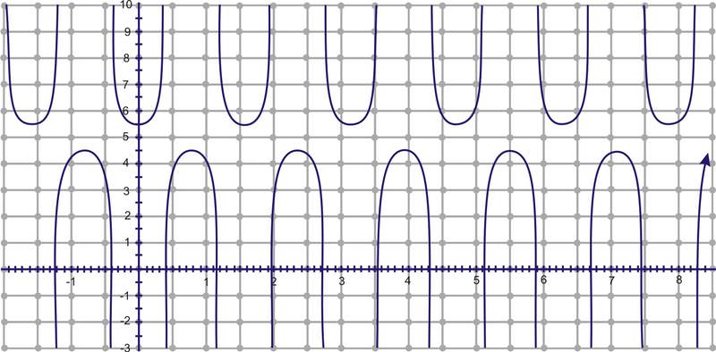
Find the equation for the graph below.
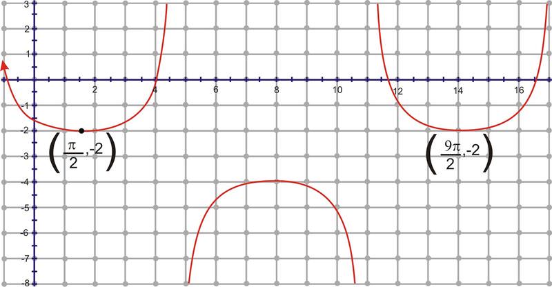
First of all, this could be either a secant or cosecant function. Let’s say this is a secant function. Secant usually intersects the y−axis at (0,1) at a minimum. Now, that corresponding minimum is \(\left(\dfrac{\pi }{2},−2\right)\). Because there is no amplitude change, we can say that the vertical shift is the difference between the two y−values, -3. It looks like there is a phase shift and a period change. From minimum to minimum is one period, which is \(\dfrac{9 \pi }{2}−\dfrac{\pi }{2}=\dfrac{8\pi }{2}=4\pi \) and \(B=\dfrac{2\pi }{4\pi} =\dfrac{1}{2}\). Lastly, we need to find the horizontal shift. Since secant usually intersects the y−axis at \((0,1)\) at a minimum, and now the corresponding minimum is \(\left(\dfrac{\pi }{2},−2\right)\), we can say that the horizontal shift is the difference between the two x−values, \(\dfrac{\pi }{2}\). Therefore, our equation is \(f(x)=−3+\sec \left(\dfrac{1}{2}\left(x−\dfrac{\pi }{2}\right)\right)\).
Graph the function \(h(x)=2−3\cos 4x\)
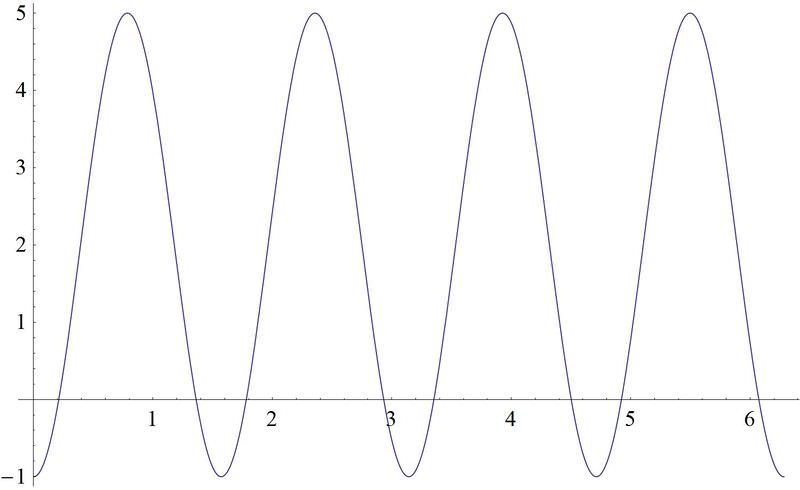
Earlier, you were asked what would the shadow trace out.
Solution
As you have learned in this section, a light shining down on the rotating hand would create a shadow in the pattern of a cosine function, starting at a maximum value as the hand is lying along the "x" axis, going through zero to a maximum negative value when the hand is lying along the negative "y" axis. It would then begin to increase until it returned to a maximum value when the rotating hand was again lying along the positive "x" axis.
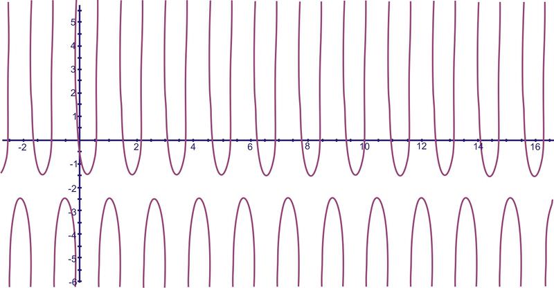
Graph \(y=−2+\dfrac{1}{2}\sec (4(x−1))\).
Solution
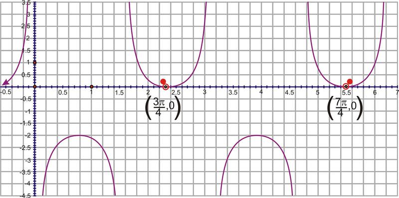
Determine the function creating this graph:
Solution
This could be either a secant or cosecant function. We will use a cosecant model. First, the vertical shift is -1. The period is the difference between the two given x−values, \(7\dfrac{\pi }{4}−\dfrac{3 \pi }{4}=\pi \), so the frequency is \(\dfrac{2\pi }{\pi }=2\). The horizontal shift incorporates the frequency, so in \(y=\csc x\) the corresponding x−value to \(\left(\dfrac{3 \pi }{4},0\right)\) is \(\left(\dfrac{\pi }{2},1\right)\). The difference between the x−values is \(\dfrac{3 \pi }{4}−\dfrac{\pi }{2}=\dfrac{3 \pi }{4}−\dfrac{2\pi }{4}=\dfrac{\pi }{4}\) and then multiply it by the frequency, \(2\cdot \dfrac{\pi }{4}=\dfrac{\pi }{2}\). The equation is \(y=−1+\csc \left(2\left(x−\dfrac{\pi }{2}\right)\right)\).
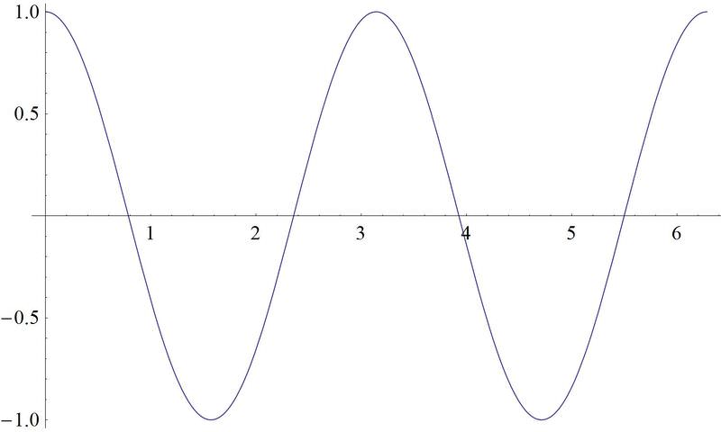
Graph \(h(x)=\dfrac{1}{3}\cos 2x\)
Solution
Review
Graph each of the following functions.
- \(f(x)=\cos (x)\).
- \(h(x)=\cos (2x)\).
- \(k(x)=\cos (2x+\pi )\).
- \(m(x)=−2\cos (2x+\pi )\).
- \(g(x)=−2\cos (2x+\pi )+1\).
- \(f(x)=\sec (x)\).
- \(h(x)=\sec (3x)\).
- \(k(x)=\sec (3x+\pi )\).
- \(m(x)=2\sec (3x+\pi )\).
- \(g(x)=3+2\sec (3x+\pi )\).
- \(h(x)=\cos \left(\dfrac{x}{2} \right )\).
- \(k(x)=\cos \left(\dfrac{x}{2}+\dfrac{\pi }{2}\right)\).
- \(m(x)=2\cos \left(\dfrac{x}{2}+\dfrac{\pi }{2}\right)\).
- \(g(x)=2\cos \left(\dfrac{x}{2}+\dfrac{\pi }{2}\right)−3\).
- \(h(x)=\sec \left(\dfrac{x}{4}\right)\).
- \(k(x)=\sec \left(\dfrac{x}{4}+\dfrac{3\pi }{2}\right)\).
- \(m(x)=−3\sec \left(\dfrac{x}{4}+\dfrac{3\pi }{2}\right)\).
- \(g(x)=2−3\sec \left(\dfrac{x}{4}+\dfrac{3\pi }{2}\right)\).
Review (Answers)
To see the Review answers, open this PDF file and look for section 2.10.
Vocabulary
| Term | Definition |
|---|---|
| Circular Function | A circular function is a function measured by examining the angle of rotation around the coordinate plane. |
Additional Resources
Video: Animation: Graphing the Cosine Function Using the Unit Circle

