3.12: Punnett Squares
- Page ID
- 1455
\( \newcommand{\vecs}[1]{\overset { \scriptstyle \rightharpoonup} {\mathbf{#1}} } \)
\( \newcommand{\vecd}[1]{\overset{-\!-\!\rightharpoonup}{\vphantom{a}\smash {#1}}} \)
\( \newcommand{\dsum}{\displaystyle\sum\limits} \)
\( \newcommand{\dint}{\displaystyle\int\limits} \)
\( \newcommand{\dlim}{\displaystyle\lim\limits} \)
\( \newcommand{\id}{\mathrm{id}}\) \( \newcommand{\Span}{\mathrm{span}}\)
( \newcommand{\kernel}{\mathrm{null}\,}\) \( \newcommand{\range}{\mathrm{range}\,}\)
\( \newcommand{\RealPart}{\mathrm{Re}}\) \( \newcommand{\ImaginaryPart}{\mathrm{Im}}\)
\( \newcommand{\Argument}{\mathrm{Arg}}\) \( \newcommand{\norm}[1]{\| #1 \|}\)
\( \newcommand{\inner}[2]{\langle #1, #2 \rangle}\)
\( \newcommand{\Span}{\mathrm{span}}\)
\( \newcommand{\id}{\mathrm{id}}\)
\( \newcommand{\Span}{\mathrm{span}}\)
\( \newcommand{\kernel}{\mathrm{null}\,}\)
\( \newcommand{\range}{\mathrm{range}\,}\)
\( \newcommand{\RealPart}{\mathrm{Re}}\)
\( \newcommand{\ImaginaryPart}{\mathrm{Im}}\)
\( \newcommand{\Argument}{\mathrm{Arg}}\)
\( \newcommand{\norm}[1]{\| #1 \|}\)
\( \newcommand{\inner}[2]{\langle #1, #2 \rangle}\)
\( \newcommand{\Span}{\mathrm{span}}\) \( \newcommand{\AA}{\unicode[.8,0]{x212B}}\)
\( \newcommand{\vectorA}[1]{\vec{#1}} % arrow\)
\( \newcommand{\vectorAt}[1]{\vec{\text{#1}}} % arrow\)
\( \newcommand{\vectorB}[1]{\overset { \scriptstyle \rightharpoonup} {\mathbf{#1}} } \)
\( \newcommand{\vectorC}[1]{\textbf{#1}} \)
\( \newcommand{\vectorD}[1]{\overrightarrow{#1}} \)
\( \newcommand{\vectorDt}[1]{\overrightarrow{\text{#1}}} \)
\( \newcommand{\vectE}[1]{\overset{-\!-\!\rightharpoonup}{\vphantom{a}\smash{\mathbf {#1}}}} \)
\( \newcommand{\vecs}[1]{\overset { \scriptstyle \rightharpoonup} {\mathbf{#1}} } \)
\(\newcommand{\longvect}{\overrightarrow}\)
\( \newcommand{\vecd}[1]{\overset{-\!-\!\rightharpoonup}{\vphantom{a}\smash {#1}}} \)
\(\newcommand{\avec}{\mathbf a}\) \(\newcommand{\bvec}{\mathbf b}\) \(\newcommand{\cvec}{\mathbf c}\) \(\newcommand{\dvec}{\mathbf d}\) \(\newcommand{\dtil}{\widetilde{\mathbf d}}\) \(\newcommand{\evec}{\mathbf e}\) \(\newcommand{\fvec}{\mathbf f}\) \(\newcommand{\nvec}{\mathbf n}\) \(\newcommand{\pvec}{\mathbf p}\) \(\newcommand{\qvec}{\mathbf q}\) \(\newcommand{\svec}{\mathbf s}\) \(\newcommand{\tvec}{\mathbf t}\) \(\newcommand{\uvec}{\mathbf u}\) \(\newcommand{\vvec}{\mathbf v}\) \(\newcommand{\wvec}{\mathbf w}\) \(\newcommand{\xvec}{\mathbf x}\) \(\newcommand{\yvec}{\mathbf y}\) \(\newcommand{\zvec}{\mathbf z}\) \(\newcommand{\rvec}{\mathbf r}\) \(\newcommand{\mvec}{\mathbf m}\) \(\newcommand{\zerovec}{\mathbf 0}\) \(\newcommand{\onevec}{\mathbf 1}\) \(\newcommand{\real}{\mathbb R}\) \(\newcommand{\twovec}[2]{\left[\begin{array}{r}#1 \\ #2 \end{array}\right]}\) \(\newcommand{\ctwovec}[2]{\left[\begin{array}{c}#1 \\ #2 \end{array}\right]}\) \(\newcommand{\threevec}[3]{\left[\begin{array}{r}#1 \\ #2 \\ #3 \end{array}\right]}\) \(\newcommand{\cthreevec}[3]{\left[\begin{array}{c}#1 \\ #2 \\ #3 \end{array}\right]}\) \(\newcommand{\fourvec}[4]{\left[\begin{array}{r}#1 \\ #2 \\ #3 \\ #4 \end{array}\right]}\) \(\newcommand{\cfourvec}[4]{\left[\begin{array}{c}#1 \\ #2 \\ #3 \\ #4 \end{array}\right]}\) \(\newcommand{\fivevec}[5]{\left[\begin{array}{r}#1 \\ #2 \\ #3 \\ #4 \\ #5 \\ \end{array}\right]}\) \(\newcommand{\cfivevec}[5]{\left[\begin{array}{c}#1 \\ #2 \\ #3 \\ #4 \\ #5 \\ \end{array}\right]}\) \(\newcommand{\mattwo}[4]{\left[\begin{array}{rr}#1 \amp #2 \\ #3 \amp #4 \\ \end{array}\right]}\) \(\newcommand{\laspan}[1]{\text{Span}\{#1\}}\) \(\newcommand{\bcal}{\cal B}\) \(\newcommand{\ccal}{\cal C}\) \(\newcommand{\scal}{\cal S}\) \(\newcommand{\wcal}{\cal W}\) \(\newcommand{\ecal}{\cal E}\) \(\newcommand{\coords}[2]{\left\{#1\right\}_{#2}}\) \(\newcommand{\gray}[1]{\color{gray}{#1}}\) \(\newcommand{\lgray}[1]{\color{lightgray}{#1}}\) \(\newcommand{\rank}{\operatorname{rank}}\) \(\newcommand{\row}{\text{Row}}\) \(\newcommand{\col}{\text{Col}}\) \(\renewcommand{\row}{\text{Row}}\) \(\newcommand{\nul}{\text{Nul}}\) \(\newcommand{\var}{\text{Var}}\) \(\newcommand{\corr}{\text{corr}}\) \(\newcommand{\len}[1]{\left|#1\right|}\) \(\newcommand{\bbar}{\overline{\bvec}}\) \(\newcommand{\bhat}{\widehat{\bvec}}\) \(\newcommand{\bperp}{\bvec^\perp}\) \(\newcommand{\xhat}{\widehat{\xvec}}\) \(\newcommand{\vhat}{\widehat{\vvec}}\) \(\newcommand{\uhat}{\widehat{\uvec}}\) \(\newcommand{\what}{\widehat{\wvec}}\) \(\newcommand{\Sighat}{\widehat{\Sigma}}\) \(\newcommand{\lt}{<}\) \(\newcommand{\gt}{>}\) \(\newcommand{\amp}{&}\) \(\definecolor{fillinmathshade}{gray}{0.9}\)
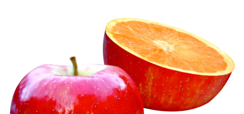
What do you get when you cross an apple and an orange?
Though the above fruit may not result, it would be nice to scientifically predict what would result. Predicting the possible genotypes and phenotypes from a genetic cross is often aided by a Punnett square.
Punnett Squares
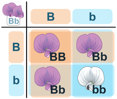
A Punnett square is a chart that allows you to easily determine the expected percentage of different genotypes in the offspring of two parents. An example of a Punnett square for pea plants is shown in the Figure below. In this example, both parents are heterozygous for flower color (Bb). The gametes produced by the male parent are at the top of the chart, and the gametes produced by the female parent are along the side. The different possible combinations of alleles in their offspring are determined by filling in the cells of the Punnett square with the correct letters (alleles).
 This Punnett square shows a cross between two heterozygotes, Bb. Do you know where each letter (allele) in all four cells comes from? Two pea plants, both heterozygous for flower color, are crossed. The offspring will show the dominant purple coloration in a 3:1 ratio. Or, about 75% of the offspring will be purple.
Predicting Offspring Genotypes
In the cross shown in the Figure above, you can see that one out of four offspring (25 percent) has the genotype BB, one out of four (25 percent) has the genotype bb, and two out of four (50 percent) have the genotype Bb. These percentages of genotypes are what you would expect in any cross between two heterozygous parents. Of course, when just four offspring are produced, the actual percentages of genotypes may vary by chance from the expected percentages. However, if you considered hundreds of such crosses and thousands of offspring, you would get very close to the expected results, just like tossing a coin.
Predicting Offspring Phenotypes
You can predict the percentages of phenotypes in the offspring of this cross from their genotypes. B is dominant to b, so offspring with either the BB or Bb genotype will have the purple-flower phenotype. Only offspring with the bb genotype will have the white-flower phenotype. Therefore, in this cross, you would expect three out of four (75 percent) of the offspring to have purple flowers and one out of four (25 percent) to have white flowers. These are the same percentages that Mendel got in his first experiment.
Determining Missing Genotypes
A Punnett square can also be used to determine a missing genotype based on the other genotypes involved in a cross. Suppose you have a parent plant with purple flowers and a parent plant with white flowers. Because the b allele is recessive, you know that the white-flowered parent must have the genotype bb. The purple-flowered parent, on the other hand, could have either the BB or the Bb genotype. The Punnett square in the Figure below shows this cross. The question marks (?) in the chart could be either B or b alleles.
 Punnett Square: Cross Between White-Flowered and Purple-Flowered Pea Plants. This Punnett square shows a cross between a white-flowered pea plant and a purple-flowered pea plant. Can you fill in the missing alleles? What do you need to know about the offspring to complete their genotypes?
Can you tell what the genotype of the purple-flowered parent is from the information in the Punnett square? No; you also need to know the genotypes of the offspring in row 2. What if you found out that two of the four offspring have white flowers? Now you know that the offspring in the second row must have the bb genotype. One of their b alleles obviously comes from the white-flowered (bb) parent, because that’s the only allele this parent has. The other b allele must come from the purple-flowered parent. Therefore, the parent with purple flowers must have the genotype Bb.
Punnett Square for Two Characteristics
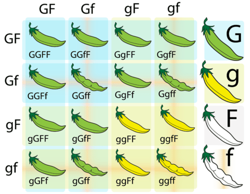
When you consider more than one characteristic at a time, using a Punnett square is more complicated. This is because many more combinations of alleles are possible. For example, with two genes each having two alleles, an individual has four alleles, and these four alleles can occur in 16 different combinations. This is illustrated for pea plants in the Figure below. In this cross, known as a dihybrid cross, both parents are heterozygous for pod color (Gg) and pod form (Ff).
 Punnett Square for Two Characteristics. This Punnett square represents a cross between two pea plants that are heterozygous for two characteristics. G represents the dominant allele for green pod color, and g represents the recessive allele for yellow pod color. F represents the dominant allele for full pod form, and f represents the recessive allele for constricted pod form.
Summary
- A Punnett square is a chart that allows you to determine the expected percentages of different genotypes in the offspring of two parents.
- A Punnett square allows the prediction of the percentages of phenotypes in the offspring of a cross from known genotypes.
- A Punnett square can be used to determine a missing genotype based on the other genotypes involved in a cross.
Review
- What is a Punnett square? How is it used?
- Draw a Punnett square of an Ss x ss cross. The S allele codes for long stems in pea plants and the s allele codes for short stems. If S is dominant to s, what percentage of the offspring would you expect to have each phenotype?
- What letter should replace the question marks (?) in this Punnett square? Explain how you know.

-
How do the Punnett squares for a monohybrid cross and a dihybrid cross differ?
- What are the genotypes of gametes of a AaBb self-pollination?
-
Mendel carried out a dihybrid cross to examine the inheritance of the characteristics for seed color and seed shape. The dominant allele for yellow seed color is Y, and the recessive allele for green color is y. The dominant allele for round seeds is R, and the recessive allele for a wrinkled shape is r. The two plants that were crossed were F1 dihybrids RrYy. Identify the ratios of traits that Mendel observed in the F2 generation. Create a Punnett square to help you answer the question.
| Image | Reference | Attributions |
 |
[Figure 1] | Credit: Mariana Ruiz Villarreal (LadyofHats) for CK-12 Foundation Source: CK-12 Foundation License: CC BY-NC |
 |
[Figure 2] | Credit: Mariana Ruiz Villarreal (LadyofHats) for CK-12 Foundation;Sam McCabe;Jodi So Source: CK-12 Foundation License: CC BY-NC 3.0 |
 |
[Figure 3] | Credit: Jodi So;Sam McCabe Source: CK-12 Foundation License: CC BY-NC 3.0 |
 |
[Figure 4] | Credit: Mariana Ruiz Villarreal (LadyofHats) for CK-12 Foundation;Sam McCabe;Jodi So Source: CK-12 Foundation License: CC BY-NC 3.0 |
 |
[Figure 5] | Credit: Mariana Ruiz Villarreal (LadyofHats) for CK-12 Foundation Source: CK-12 Foundation License: CC BY-NC |

