
9.2: p-Values
- Page ID
- 5784
\( \newcommand{\vecs}[1]{\overset { \scriptstyle \rightharpoonup} {\mathbf{#1}} } \)
\( \newcommand{\vecd}[1]{\overset{-\!-\!\rightharpoonup}{\vphantom{a}\smash {#1}}} \)
\( \newcommand{\dsum}{\displaystyle\sum\limits} \)
\( \newcommand{\dint}{\displaystyle\int\limits} \)
\( \newcommand{\dlim}{\displaystyle\lim\limits} \)
\( \newcommand{\id}{\mathrm{id}}\) \( \newcommand{\Span}{\mathrm{span}}\)
( \newcommand{\kernel}{\mathrm{null}\,}\) \( \newcommand{\range}{\mathrm{range}\,}\)
\( \newcommand{\RealPart}{\mathrm{Re}}\) \( \newcommand{\ImaginaryPart}{\mathrm{Im}}\)
\( \newcommand{\Argument}{\mathrm{Arg}}\) \( \newcommand{\norm}[1]{\| #1 \|}\)
\( \newcommand{\inner}[2]{\langle #1, #2 \rangle}\)
\( \newcommand{\Span}{\mathrm{span}}\)
\( \newcommand{\id}{\mathrm{id}}\)
\( \newcommand{\Span}{\mathrm{span}}\)
\( \newcommand{\kernel}{\mathrm{null}\,}\)
\( \newcommand{\range}{\mathrm{range}\,}\)
\( \newcommand{\RealPart}{\mathrm{Re}}\)
\( \newcommand{\ImaginaryPart}{\mathrm{Im}}\)
\( \newcommand{\Argument}{\mathrm{Arg}}\)
\( \newcommand{\norm}[1]{\| #1 \|}\)
\( \newcommand{\inner}[2]{\langle #1, #2 \rangle}\)
\( \newcommand{\Span}{\mathrm{span}}\) \( \newcommand{\AA}{\unicode[.8,0]{x212B}}\)
\( \newcommand{\vectorA}[1]{\vec{#1}} % arrow\)
\( \newcommand{\vectorAt}[1]{\vec{\text{#1}}} % arrow\)
\( \newcommand{\vectorB}[1]{\overset { \scriptstyle \rightharpoonup} {\mathbf{#1}} } \)
\( \newcommand{\vectorC}[1]{\textbf{#1}} \)
\( \newcommand{\vectorD}[1]{\overrightarrow{#1}} \)
\( \newcommand{\vectorDt}[1]{\overrightarrow{\text{#1}}} \)
\( \newcommand{\vectE}[1]{\overset{-\!-\!\rightharpoonup}{\vphantom{a}\smash{\mathbf {#1}}}} \)
\( \newcommand{\vecs}[1]{\overset { \scriptstyle \rightharpoonup} {\mathbf{#1}} } \)
\(\newcommand{\longvect}{\overrightarrow}\)
\( \newcommand{\vecd}[1]{\overset{-\!-\!\rightharpoonup}{\vphantom{a}\smash {#1}}} \)
\(\newcommand{\avec}{\mathbf a}\) \(\newcommand{\bvec}{\mathbf b}\) \(\newcommand{\cvec}{\mathbf c}\) \(\newcommand{\dvec}{\mathbf d}\) \(\newcommand{\dtil}{\widetilde{\mathbf d}}\) \(\newcommand{\evec}{\mathbf e}\) \(\newcommand{\fvec}{\mathbf f}\) \(\newcommand{\nvec}{\mathbf n}\) \(\newcommand{\pvec}{\mathbf p}\) \(\newcommand{\qvec}{\mathbf q}\) \(\newcommand{\svec}{\mathbf s}\) \(\newcommand{\tvec}{\mathbf t}\) \(\newcommand{\uvec}{\mathbf u}\) \(\newcommand{\vvec}{\mathbf v}\) \(\newcommand{\wvec}{\mathbf w}\) \(\newcommand{\xvec}{\mathbf x}\) \(\newcommand{\yvec}{\mathbf y}\) \(\newcommand{\zvec}{\mathbf z}\) \(\newcommand{\rvec}{\mathbf r}\) \(\newcommand{\mvec}{\mathbf m}\) \(\newcommand{\zerovec}{\mathbf 0}\) \(\newcommand{\onevec}{\mathbf 1}\) \(\newcommand{\real}{\mathbb R}\) \(\newcommand{\twovec}[2]{\left[\begin{array}{r}#1 \\ #2 \end{array}\right]}\) \(\newcommand{\ctwovec}[2]{\left[\begin{array}{c}#1 \\ #2 \end{array}\right]}\) \(\newcommand{\threevec}[3]{\left[\begin{array}{r}#1 \\ #2 \\ #3 \end{array}\right]}\) \(\newcommand{\cthreevec}[3]{\left[\begin{array}{c}#1 \\ #2 \\ #3 \end{array}\right]}\) \(\newcommand{\fourvec}[4]{\left[\begin{array}{r}#1 \\ #2 \\ #3 \\ #4 \end{array}\right]}\) \(\newcommand{\cfourvec}[4]{\left[\begin{array}{c}#1 \\ #2 \\ #3 \\ #4 \end{array}\right]}\) \(\newcommand{\fivevec}[5]{\left[\begin{array}{r}#1 \\ #2 \\ #3 \\ #4 \\ #5 \\ \end{array}\right]}\) \(\newcommand{\cfivevec}[5]{\left[\begin{array}{c}#1 \\ #2 \\ #3 \\ #4 \\ #5 \\ \end{array}\right]}\) \(\newcommand{\mattwo}[4]{\left[\begin{array}{rr}#1 \amp #2 \\ #3 \amp #4 \\ \end{array}\right]}\) \(\newcommand{\laspan}[1]{\text{Span}\{#1\}}\) \(\newcommand{\bcal}{\cal B}\) \(\newcommand{\ccal}{\cal C}\) \(\newcommand{\scal}{\cal S}\) \(\newcommand{\wcal}{\cal W}\) \(\newcommand{\ecal}{\cal E}\) \(\newcommand{\coords}[2]{\left\{#1\right\}_{#2}}\) \(\newcommand{\gray}[1]{\color{gray}{#1}}\) \(\newcommand{\lgray}[1]{\color{lightgray}{#1}}\) \(\newcommand{\rank}{\operatorname{rank}}\) \(\newcommand{\row}{\text{Row}}\) \(\newcommand{\col}{\text{Col}}\) \(\renewcommand{\row}{\text{Row}}\) \(\newcommand{\nul}{\text{Nul}}\) \(\newcommand{\var}{\text{Var}}\) \(\newcommand{\corr}{\text{corr}}\) \(\newcommand{\len}[1]{\left|#1\right|}\) \(\newcommand{\bbar}{\overline{\bvec}}\) \(\newcommand{\bhat}{\widehat{\bvec}}\) \(\newcommand{\bperp}{\bvec^\perp}\) \(\newcommand{\xhat}{\widehat{\xvec}}\) \(\newcommand{\vhat}{\widehat{\vvec}}\) \(\newcommand{\uhat}{\widehat{\uvec}}\) \(\newcommand{\what}{\widehat{\wvec}}\) \(\newcommand{\Sighat}{\widehat{\Sigma}}\) \(\newcommand{\lt}{<}\) \(\newcommand{\gt}{>}\) \(\newcommand{\amp}{&}\) \(\definecolor{fillinmathshade}{gray}{0.9}\)What are critical values? Why is it important to know if a test is left, right, or two-tailed, when calculating critical values?
Critical Values
When you calculate the probability that a range of values will occur given a random variable with a particular distribution, you often use a z-score reference or calculator.
Critical values are the values that indicate the edge of the critical region. Critical regions (also known as rejection regions) describe the entire area of values that indicate you reject the null hypothesis. In other words, the critical region is the area encompassed by the values not supportive of the default assumption - the area of the ‘tails’ of the distribution.
In this lesson, we will use a table to find critical values. Although critical values may refer to other types of distributions, for the moment we will be dealing only with the Z-score critical values of a normal distribution. There is a table of Z-score values that you may refer to here:
| Z | 0.00 | 0.01 | 0.02 | 0.03 | 0.04 | 0.05 | 0.06 | 0.07 | 0.08 | 0.09 | Z |
| 0.0 |
0.5 |
0.504 |
0.508 |
0.512 |
0.516 |
0.5199 |
0.5239 |
0.5279 |
0.5319 |
0.5359 |
0.0 |
| 0.1 |
0.5398 |
0.5438 |
0.5478 |
0.5517 |
0.5557 |
0.5596 |
0.5636 |
0.5675 |
0.5714 |
0.5753 |
0.1 |
| 0.2 |
0.5793 |
0.5832 |
0.5871 |
0.591 |
0.5948 |
0.5987 |
0.6026 |
0.6064 |
0.6103 |
0.6141 |
0.2 |
| 0.3 |
0.6179 |
0.6217 |
0.6255 |
0.6293 |
0.6331 |
0.6368 |
0.6406 |
0.6443 |
0.648 |
0.6517 |
0.3 |
| 0.4 |
0.6554 |
0.6591 |
0.6628 |
0.6664 |
0.67 |
0.6736 |
0.6772 |
0.6808 |
0.6844 |
0.6879 |
0.4 |
| 0.5 |
0.6915 |
0.695 |
0.6985 |
0.7019 |
0.7054 |
0.7088 |
0.7123 |
0.7157 |
0.719 |
0.7224 |
0.5 |
| 0.6 |
0.7257 |
0.7291 |
0.7324 |
0.7357 |
0.7389 |
0.7422 |
0.7454 |
0.7486 |
0.7517 |
0.7549 |
0.6 |
| 0.7 |
0.758 |
0.7611 |
0.7642 |
0.7673 |
0.7704 |
0.7734 |
0.7764 |
0.7794 |
0.7823 |
0.7852 |
0.7 |
| 0.8 |
0.7881 |
0.791 |
0.7939 |
0.7967 |
0.7995 |
0.8023 |
0.8051 |
0.8078 |
0.8106 |
0.8133 |
0.8 |
| 0.9 |
0.8159 |
0.8186 |
0.8212 |
0.8238 |
0.8264 |
0.8289 |
0.8315 |
0.834 |
0.8365 |
0.8389 |
0.9 |
| 1.0 |
0.8413 |
0.8438 |
0.8461 |
0.8485 |
0.8508 |
0.8531 |
0.8554 |
0.8577 |
0.8599 |
0.8621 |
1.0 |
| 1.1 |
0.8643 |
0.8665 |
0.8686 |
0.8708 |
0.8729 |
0.8749 |
0.877 |
0.879 |
0.881 |
0.883 |
1.1 |
| 1.2 |
0.8849 |
0.8869 |
0.8888 |
0.8907 |
0.8925 |
0.8944 |
0.8962 |
0.898 |
0.8997 |
0.9015 |
1.2 |
| 1.3 |
0.9032 |
0.9049 |
0.9066 |
0.9082 |
0.9099 |
0.9115 |
0.9131 |
0.9147 |
0.9162 |
0.9177 |
1.3 |
| 1.4 |
0.9192 |
0.9207 |
0.9222 |
0.9236 |
0.9251 |
0.9265 |
0.9279 |
0.9292 |
0.9306 |
0.9319 |
1.4 |
| 1.5 |
0.9332 |
0.9345 |
0.9357 |
0.937 |
0.9382 |
0.9394 |
0.9406 |
0.9418 |
0.9429 |
0.9441 |
1.5 |
| 1.6 |
0.9452 |
0.9463 |
0.9474 |
0.9484 |
0.9495 |
0.9505 |
0.9515 |
0.9525 |
0.9535 |
0.9545 |
1.6 |
| 1.7 |
0.9554 |
0.9564 |
0.9573 |
0.9582 |
0.9591 |
0.9599 |
0.9608 |
0.9616 |
0.9625 |
0.9633 |
1.7 |
| 1.8 |
0.9641 |
0.9649 |
0.9656 |
0.9664 |
0.9671 |
0.9678 |
0.9686 |
0.9693 |
0.9699 |
0.9706 |
1.8 |
| 1.9 |
0.9713 |
0.9719 |
0.9726 |
0.9732 |
0.9738 |
0.9744 |
0.975 |
0.9756 |
0.9761 |
0.9767 |
1.9 |
| 2.0 |
0.9772 |
0.9778 |
0.9783 |
0.9788 |
0.9793 |
0.9798 |
0.9803 |
0.9808 |
0.9812 |
0.9817 |
2.0 |
| 2.1 |
0.9821 |
0.9826 |
0.983 |
0.9834 |
0.9838 |
0.9842 |
0.9846 |
0.985 |
0.9854 |
0.9857 |
2.1 |
| 2.2 |
0.9861 |
0.9864 |
0.9868 |
0.9871 |
0.9875 |
0.9878 |
0.9881 |
0.9884 |
0.9887 |
0.989 |
2.2 |
| 2.3 |
0.9893 |
0.9896 |
0.9898 |
0.9901 |
0.9904 |
0.9906 |
0.9909 |
0.9911 |
0.9913 |
0.9916 |
2.3 |
| 2.4 |
0.9918 |
0.992 |
0.9922 |
0.9925 |
0.9927 |
0.9929 |
0.9931 |
0.9932 |
0.9934 |
0.9936 |
2.4 |
| 2.5 |
0.9938 |
0.994 |
0.9941 |
0.9943 |
0.9945 |
0.9946 |
0.9948 |
0.9949 |
0.9951 |
0.9952 |
2.5 |
| 2.6 |
0.9953 |
0.9955 |
0.9956 |
0.9957 |
0.9959 |
0.996 |
0.9961 |
0.9962 |
0.9963 |
0.9964 |
2.6 |
| 2.7 |
0.9965 |
0.9966 |
0.9967 |
0.9968 |
0.9969 |
0.997 |
0.9971 |
0.9972 |
0.9973 |
0.9974 |
2.7 |
| 2.8 |
0.9974 |
0.9975 |
0.9976 |
0.9977 |
0.9977 |
0.9978 |
0.9979 |
0.9979 |
0.998 |
0.9981 |
2.8 |
| 2.9 |
0.9981 |
0.9982 |
0.9982 |
0.9983 |
0.9984 |
0.9984 |
0.9985 |
0.9985 |
0.9986 |
0.9986 |
2.9 |
| 3.0 |
0.9987 |
0.9987 |
0.9987 |
0.9988 |
0.9988 |
0.9989 |
0.9989 |
0.9989 |
0.999 |
0.999 |
3.0 |
| 3.1 |
0.999 |
0.9991 |
0.9991 |
0.9991 |
0.9992 |
0.9992 |
0.9992 |
0.9992 |
0.9993 |
0.9993 |
3.1 |
| 3.2 |
0.9993 |
0.9993 |
0.9994 |
0.9994 |
0.9994 |
0.9994 |
0.9994 |
0.9995 |
0.9995 |
0.9995 |
3.2 |
| 3.3 |
0.9995 |
0.9995 |
0.9995 |
0.9996 |
0.9996 |
0.9996 |
0.9996 |
0.9996 |
0.9996 |
0.9997 |
3.3 |
| 3.4 |
0.9997 |
0.9997 |
0.9997 |
0.9997 |
0.9997 |
0.9997 |
0.9997 |
0.9997 |
0.9997 |
0.9998 |
3.4 |
| 3.5 |
0.9998 |
0.9998 |
0.9998 |
0.9998 |
0.9998 |
0.9998 |
0.9998 |
0.9998 |
0.9998 |
0.9998 |
3.5 |
| 3.6 |
0.9998 |
0.9998 |
0.9999 |
0.9999 |
0.9999 |
0.9999 |
0.9999 |
0.9999 |
0.9999 |
0.9999 |
3.6 |
| 3.7 |
0.9999 |
0.9999 |
0.9999 |
0.9999 |
0.9999 |
0.9999 |
0.9999 |
0.9999 |
0.9999 |
0.9999 |
3.7 |
| 3.8 |
0.9999 |
0.9999 |
0.9999 |
0.9999 |
0.9999 |
0.9999 |
0.9999 |
0.9999 |
0.9999 |
0.9999 |
3.8 |
| 3.9 |
1 |
1 |
1 |
1 |
1 |
1 |
1 |
1 |
1 |
1 |
3.9 |
| Z | 0.00 | 0.01 | 0.02 | 0.03 | 0.04 | 0.05 | 0.06 | 0.07 | 0.08 | 0.09 | Z |
In the next lesson, we will discuss how to identify a test as Left, Right, or Two-tailed. For now, the problems will specify which type you are working with since it affects the location of the critical value(s), and therefore the area of the critical region.
If you have completed the prior lesson(s) on Z-scores, you should recognize Z-score critical values as the Z-scores associated with a given percentage. The reason there is another term, critical values, instead of just Z-scores, is that the concept of critical values is also applicable to other types of distributions, such as the student’s t-score distribution discussed in the lesson Degrees of Freedom.
Determining Critical Values
What is the critical value (Zαz) for a 95% confidence level, assuming a two-tailed test?
A 95% confidence level means that a total of 5% of the area under the curve is considered the critical region.
Since this is a two-tailed test, 12 of 5%=2.5% of the values would be in the left tail, and the other 2.5% would be in the right tail. Looking up the Z-score associated with 0.025 on a reference table, we find 1.96. Therefore, +1.96 is the critical value of the right tail and -1.96 is the critical value of the left tail.
The critical value for a 95% confidence level is Z=+/−1.96.
Sketching the Z-Score
Sketch the Z-score critical region for the previous example.
Sketch the graph of the normal distribution with the given values and mark the critical values from Ex. A, then shade the area from the critical values away from the center. The shaded areas are the critical regions.

CC BY-NC-SA
Finding the Critical Value
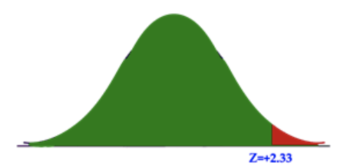
What would be the critical value for a right-tailed test with α=0.01?
If α=0.01, then the area under the curve representing H1, the alternative hypothesis, would be 99%, since α (alpha) is the same as the area of the rejection region. Using the Z-score reference table above, we find that the Z-score associated with 0.9900 is approximately 2.33.
It appears that the critical value is Z=2.33.
Let’s see if that answer makes sense. Since this is a right-tailed test, α is on the right end of the graph, and 1−α is on the left. A Z-score of +2.33 is well to the right of the center of the graph, splitting the area under the curve from that point to the left, and indicating that the values supporting the default hypothesis encompass nearly the entire graph. Since the initial question specified α=0.01, indicating that only 1% of the area is in the critical region, Z=+2.33 is quite reasonable.
CC BY-NC-SA
Earlier Problem Revisited
What are critical values? Why is it important to know if a test is left, right, or two-tailed, when calculating critical values?
Critical values are the values which separate the area indicating the null hypothesis should be rejected from the area suggesting it not be rejected. It is important to know what kind of test you are dealing with, because the critical value is often calculated from a probability range, and the Z-score of that range changes depending on what portion of the distribution you are evaluating.
Vocabulary
Critical values are values separating the values that support or reject the null hypothesis.
Critical regions are the areas under the distribution curve representing values that support the null hypothesis.
Examples
Example 1
What would be the critical value for a left-tailed test with α=0.01?
A left-tailed test with α=0.01 would have 99% of the area under the curve outside of the critical region. If we use a reference to find the Z-score for 0.99, we get approximately 2.33. However, a Z-score of 2.33 is significantly to the right of the center of the distribution, including all the area to the left and only leaving a very small alpha value on the right. While we are indeed looking for a critical value with only a very small alpha, this is a left-tailed test, so the critical value we need is negative.
Z=−2.33
Example 2
What would be the critical region for a two-tailed test with α=0.08?
We are looking for the critical region here, but let’s start by finding the critical values. This is a two-tailed test, so half of the alpha will be in the left tail, and half in the right. That means that we are looking for a positive/negative critical value associated with an alpha of 0.04, which indicates that we need to find the Z-score for (1−0.04)=0.96. Referring to the Z-score table, we see that 0.96 corresponds to approximately 1.75. The critical values, then are +/- 1.75, and the critical region would be Z<−1.75∪Z>1.75.
Example 3
What would be the α for a right-tailed test with a critical value of Z=1.76?
The area under the curve associated with a Z-score of 1.76, according to the reference table above, is 0.9608. Since 96.08% of the area is to the left of Z=1.76, that leaves approximately 1−0.9608=0.0392 as the area in the critical region.
α=0.0392
Review
For questions 1-9, identify the critical value(s) for each α:
1. α=0.05, left-tailed
2. α=0.02, right-tailed
3. α=0.05, two-tailed
4. α=0.02, left-tailed
5. α=0.01, right-tailed
6. α=0.01, two-tailed
7. α=0.1, left-tailed
8. α=0.1, right-tailed
9. α=0.1, two-tailed
For questions 10-15, find α for the given critical value(s):
10. Z=1.28, right-tailed
11. Z=1.65,−1.65
12. Z=−3.10, left-tailed
13. Z=2.58,−2.58
14. Z=−1.65, left-tailed
15. Z=2.33, right-tailed
Vocabulary
| Term | Definition |
|---|---|
| confidence intervals | A confidence interval is an interval within which you expect to capture a specific value. The confidence interval width is dependent on the confidence level. |
| critical regions | Critical regions (or rejection regions) describe the entire area of values that indicate you reject the null hypothesis. |
| critical values | Critical values are the values that indicate the edge of the critical region. |
| level of significance | The numerical measure that we use to determine the strength of the sample evidence we are willing to consider strong enough to reject H0 is called the level of significance and it is denoted by alpha. |
| p-value | A p-value is a probability of obtaining a test statistic at least as extreme as the one that was observed, assuming that Ho is true. |
| power of the test | The power of a test is defined as the probability of rejecting the null hypothesis when it is false (that is, making the correct decision). |
| single tailed hypothesis test | A single-tail hypothesis test also means that we have only one critical region because we put the entire region of rejection into just one side of the distribution. |
| two-tailed test | A two-tailed test has tails on both ends of the normal distribution curve. The null hypothesis will be in the form Ho = 5, for example. |
| Type I error | A Type I error occurs when a true null hypothesis is rejected. |
| Type II error | A Type II error occurs when a false null hypothesis is not rejected. |
| z-score | The z -score of a value is the number of standard deviations between the value and the mean of the set. |
Additional Resources
Video: Understanding the P-Value
Practice: p-Values