1.1: 1.1 Function Families

Functions come in all different shapes. A few are very closely related and others are very different, but often confused. For example, what is the difference between \(x^{2}\) and \(2^{x}\)? They both have an \(x\) and a 2 and they both equal 4 when \(x=2\), but one eventually becomes much bigger than the other.

Families of Functions

If mathematicians are cooks, then families of functions are their ingredients. Each family of functions has its own flavor and personality. Before you learn to combine functions to create an infinite number of potential models, you need to get a clear idea of the name of each function family and how it acts.

The Identity Function: \(f(x)=x\)

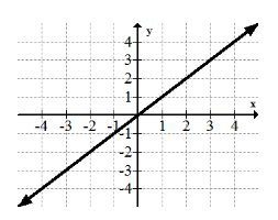
The identity function is the simplest function and all straight lines are transformations of the identity function family.

The Squaring Function: \(f(x)=x^{2}\)

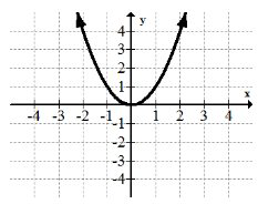
The squaring function(quadratic function) is commonly called a parabola and is useful for modeling the motion of falling objects. All parabolas are transformations of this squaring function.

The Cubing Function: \(f(x)=x^{3}\)

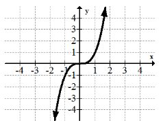
The cubing function has a different kind of symmetry than the squaring function. Since volume is measured in cubic units, many physics applications use the cubic function.

The Square Root Function: \(f(x)=\sqrt{x}=x^{\frac{1}{2}}\)

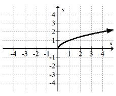
The square root function is not defined over all real numbers. It introduces the possibility of complex numbers and is also closely related to the squaring function.

The Reciprocal Function: \(f(x)=x^{-1}=\frac{1}{x}\)

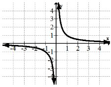
The reciprocal function is also known as a hyperbola and a rational function. It has two parts that are disconnected and is not defined at zero. Simple electric circuits are modeled with the reciprocal function.

So far all the functions can be grouped together into an even larger function family called the power function family.

The Power Function Family: \(f(x)=c x^{a}\)

The power function family has two parameters. The parameter \(c\) is a vertical scale factor. The parameter \(a\) controls everything about the shape. The reason why all the functions so far are subsets of the larger power function family is because they only differ in their value of \(a\). The power function family also shows you that there are an infinite number of other functions like quartics \(\left(f(x)=x^{4}\right)\) and quintics \(\left(f(x)=x^{5}\right)\) that don’t really need a whole category of their own. The power function family can be extended to create polynomials and rational functions.

The Exponential Function Family: \(f(x)=e^{x}\)

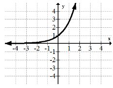
The exponential function family is one of the first functions you see where \(x\) is not the base of the exponent. This function eventually grows much faster than any power function. \(f(x)=2^{x}\) is a very common exponential function as well. Many applications like biology and finance require the use of exponential growth.

The Logarithm Function: \(f(x)=\ln x\)

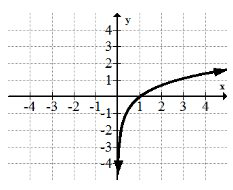
The logarithmic function is closely related to the exponential function family. Many people confuse the graph of the log function with the square root function. Careful analysis will show several important differences. The log function is the basis for the Richter Scale which is how earthquakes are measured.

The Periodic Function Family: \(f(x)=\sin x\)

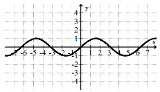
The sine graph is one of many periodic functions. Periodic refers to the fact that the sine wave repeats a cycle every period of time. Periodic functions are extremely important for modeling tides and other real world phenomena.

The Absolute Value Function: \(f(x)=|x|\)

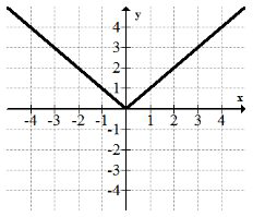
The absolute value function is one of the few basic functions that is not totally smooth.

The Logistic Function: \(f(x)=\frac{1}{1+e^{-x}}\)

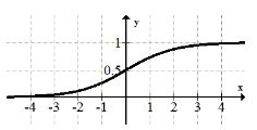
The logistic function is a combination of the exponential function and the reciprocal function. This curve is very powerful because it models population growths where the maximum population is limited by environmental resources.

Examples

Example 1

Earlier, you were given a problem about comparing \(x^{2}\) and \(2^{x}\). While \(x^{2}\) and \(2^{x}\) have similar ingredients, they have very different graphical features. The squaring function is symmetric about the line \(x=0\) while the exponential function is not. When \(x=0\), the squaring function has a height of zero and the exponential function has a height of one. The squaring function has a slope that becomes steeper as \(x\) gets further from the origin while the exponential function flattens as \(x\) gets very small. All of these differences are important and not obvious at first glance.

Example 2

\(y=x\), \(y=e^{x}\), \(y=\frac{1}{1+e^{-x}} .\) Some functions that are close but not quite: \(y=x^{3}\), \(y=\sqrt{x}\)

Example 3

Compare and contrast the graphs of the two functions:

\(f(x)=\ln x\) and \(h(x)=\sqrt{x}\)

Similarities: Both functions increase without bound as \(x\) gets larger. Both functions are not defined for negative numbers.

Differences: The log function approaches negative infinity as \(x\) approaches 0. The square root function, on the other hand, just ends at the point (0,0).

Example 4

Describe the symmetry among the function families discussed in this concept. Consider both reflection symmetry and rotational symmetry.

Some function families have reflective symmetry with themselves:

\(y=x\), \(y=x^{2}\), \(y=\frac{1}{x}\), \(y=|x|\)

Some function families are rotationally symmetric:

\(y=x\), \(y=x^{3}\), \(y=\frac{1}{x}\), \(y=\sin x\), \(y=\frac{1}{1+e^{-x}}\)

Some pairs of function families are full or partial reflections of other function families:

\(y=x^{2}\), \(y=\sqrt{x}\)

\(y=e^{x}\), \(y=\ln x\)

Review

For 1-10, sketch a graph of the function from memory.

1. \(y=e^{x}\)

2. \(y=\ln (x)\)

3. \(y=\sin (x)\)

4. \(y=x^{2}\)

5. \(y=|x|\)

6. \(y=\frac{1}{x}\)

7. \(y=\frac{1}{1+e^{-x}}\)

8. \(y=\sqrt{x}\)

9. \(y=x^{3}\)

10. \(y=x\)

11. Which function is not defined at 0? Why?

12. Which functions are bounded below but not above??

13. What are the differences between \(y=x^{2}\) and \(y=x^{3}\)?

14. What is a similarity between \(y=e^{x}\) and \(y=\ln (x)\)?

15. Explain why \(y=\sqrt{x}\) is not defined for all values of \(x\).