1.2: 1.2 Graphical Transformations

The basic functions are powerful, but they are extremely limited until you can change them to match any given situation. Transformation means that you can change the equation of a basic function by adding, subtracting, and/or multiplying by constants and thus cause a corresponding change in the graph. What are the effects of the following transformations?

1. \(f(x) \rightarrow f(x+3)\)
2. \(h(x) \rightarrow h(x)-5\)
3. \(g(x) \rightarrow-g(2 x)\)
4. \(j(x) \rightarrow j\left(-\frac{x}{2}\right)\)

Transforming Functions

A function is a rule that takes any input \(x\) and gives a specific output. When you use letters like \(f\), \(g\), \(h\), or \(j\) to describe the rule, this is called function notation. In order to interpret what effect the algebraic change in the equation will have on the graph, it is important to be able to read those changes in general function notation and then apply them to specific cases.

When transforming a function, you can transform the argument (the part inside the parentheses with the \(x\)), or the function itself. There are two ways to linearly transform the argument. You can multiply the \(x\) by a constant and/or add a constant to the \(x\) as shown below:

\(f(x) \rightarrow f(b x+c)\)

The function itself can also be linearly transformed in the same ways:

\(f(x) \rightarrow a f(x)+d\)

Each of the letters \(a\),\(b\),\(c\), and \(d\) corresponds to a very specific change. Some of these changes are straightforward, while others may be the opposite of what you might expect.

• \(a\) is a vertical stretch. If \(a\) is negative, there is also a reflection across the \(x\) axis.
• \(d\) is a vertical shift. If \(d\) is positive, then the shift is up. If \(d\) is negative, then the shift is down.

When transforming the argument of the function things are more complicated.

• \(\frac{1}{b}\) is a horizontal stretch. If \(b\) is negative, there is also a reflection across the \(y\) axis.
• \(c\) is a horizontal shift. If \(c\) is positive, then the shift is to the left. If \(c\) is negative, then the shift is to the right. Notice that this is the opposite of what most people think at first.

The trickiest part with transforming the argument of a function is the order in which you carry out the transformations. Often it makes sense to apply the transformation to a specific function that is known and then describe the transformation that you see.

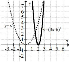
The graph below shows the transformation \(f(x) \rightarrow f(3 x-6)\) applied to a simple parabola:

Clearly the graph is narrower and to the right, but in order to be specific you must look closer. First, notice that the transformation is entirely within the argument of the function. This affects only the horizontal values. This means while the graph seems like it was stretched vertically, you must keep your perspective focused on a horizontal compression.

Look carefully at the vertex of the parabola. It has moved to the right two units. This is because first the entire graph was shifted entirely to the right 6 units. Then the function was horizontally compressed by a factor of 3 which means the point (6, 0) became (2, 0) and the \(x\) value of every other point was also compressed by a factor of 3 towards the line \(x=0\). This method is counter-intuitive because it requires reading the transformations backwards (the opposite of the way the order of operations tells you to).

Alternatively, the argument can be factored and each component of the transformation will present itself.

\(f(3(x-2))\)

This time the stretch occurs from the center of the transformed graph, not the origin. This method is ultimately the preferred method.

Either way, this is a horizontal compression by a factor of 3 and a horizontal shift to the right by 2 units.

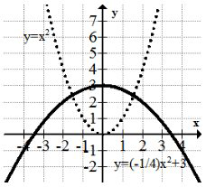
Now take the transformation \(f(x) \rightarrow-\frac{1}{4} f(x)+3 .\) It describes a vertical stretch by a factor of \(\frac{1}{4},\) a reflection over the \(x\) axis, and a vertical shift 3 units up. As opposed to what you saw above, the order of the transformations for anything outside of the argument is directly what the order of operations dictates.

First, the parabola is reflected over the \(x\) axis and compressed vertically so it appears wider. Then, every point is moved up 3 units.

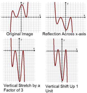
The transformation \(f(x) \rightarrow-3 f\left(-\frac{1}{2} x-1\right)+1\) contains every possible transformation. The horizontal and the vertical components do not interact with each other and so your description of the transformation can begin with either component. Here, start by describing the vertical components of the transformation:

First, there is reflection across the \(x\) axis and a vertical stretch by a factor of 3. Then, there is a vertical shift up 1 unit. Below is an image of a non-specific function going through the vertical transformations.

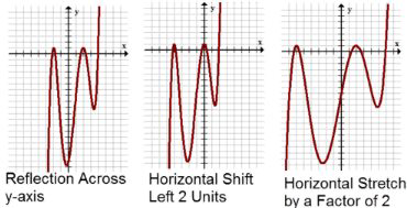
In order to figure out the horizontal components of the transformation, start by factoring the inside of the parentheses (the argument):

\(f\left(-\frac{1}{2} x-1\right)=f\left(-\frac{1}{2}(x+2)\right)\)

Factoring reveals a reflection across the \(y\) axis, a horizontal shift left 2 units and a horizontal stretch by a factor of \(2 .\) Below is an image of the same function going through the horizontal transformations.

Examples

Example 1

Earlier, you were given a problem about the effects of the following transformations:

\(f(x) \rightarrow f(x+3)\)

This transformation shifts the entire graph left 3 units. A common misconception is to shift right because the three is positive.

\(h(x) \rightarrow h(x)-5\)

This transformation shifts the entire graph down 5 units.

\(g(x) \rightarrow-g(2 x)\)

This transformation is a vertical reflection across the x axis and a horizontal compression by a factor of 2.

\(j(x)=j\left(-\frac{x}{2}\right)\)

This transformation is a horizontal reflection across the \(y\) axis and a horizontal stretch by a factor of \(2 .\) A common misconception is to see the \(\frac{1}{2}\) and believe that the \(x\) values will be half as big which is a horizontal compression. However, the \x\) values need to be twice as big to counteract this factor of \(\frac{1}{2}\)

Example 2

Describe the following transformation in words: \(g(x) \rightarrow 2 g(-x)\)

Vertical stretch by a factor of 2 and a reflection across the \(y\) axis.

Example 3

Describe the transformation that would change \(h(x)\) in the following ways:

• Vertical compression by a factor of 3.
• Vertical shift down 4 units.
• Horizontal shift right 5 units.

\(\frac{1}{3} h(x-5)-4\)

Example 4

Describe the transformation that would change \(f(x)\) in the following ways:

• Horizontal stretch by a factor of 4 and a horizontal shift 3 units to the right.
• Vertical reflection across the \(x\) axis and a shift down 2 units.

\(-f\left(\frac{1}{4}(x-3)\right)-2\) or \(-f\left(\frac{1}{4} x-\frac{3}{4}\right)-2\)

Review

Describe the following transformations in words.

1. \(g(x) \rightarrow-g(-x)\)
2. \(f(x) \rightarrow-f(x+3)\)
3. \(h(x) \rightarrow h(x+1)-2\)
4. \(j(x) \rightarrow j(-x+3)\)
5. \(k(x) \rightarrow-k(2 x)\)
6. \(f(x) \rightarrow 4 f\left(\frac{1}{2} x+1\right)\)
7. \(g(x) \rightarrow-3 g(x-2)-2\)
8. \(h(x) \rightarrow 5 h(x+1)\)

9. Describe the transformation that would change \(h(x)\) in the following
ways:

• Vertical stretch by a factor of 2
• Vertical shift up 3 units.
• Horizontal shift right 2 units.

10. Describe the transformation that would change \(f(x)\) in the following
ways:

• Vertical reflection across the x axis.
• Vertical shift down 1 unit.
• Horizontal shift left 2 units.

11. Describe the transformation that would change \(g(x)\) in the following
ways:

• Vertical compression by a factor of 4.
• Reflection across the \(y\) axis.

12. Describe the transformation that would change \(j(x)\) in the following
ways:

• Horizontal compression by a factor of 3.
• Vertical shift up 3 units.
• Horizontal shift right 2 units.

13. Describe the transformation that would change \(k(x)\) in the following
ways:

• Horizontal stretch by a factor of 4.
• Vertical shift up 3 units.
• Horizontal shift left 1 unit.

14. Describe the transformation that would change \(h(x)\) in the following
ways:

• Vertical compression by a factor of 2.
• Horizontal shift right 3 units.
• Reflection across the \(y\) axis.

15. Describe the transformation that would change \(f(x)\) in the following
ways:

• Vertical stretch by a factor of 5.
• Reflection across the \(x\) axis