9.13: ANOVA Tests

Two-Way ANOVA Tests 

In a previous Concept, we discussed the one-way ANOVA method, which is the procedure for testing the null hypothesis that the population means and variances of a single independent variable are equal.

Testing the Means and Variances of Multiple Independent Variables

Sometimes, however, we are interested in testing the means and variances of more than one independent variable. Say, for example, that a researcher is interested in determining the effects of different dosages of a dietary supplement on the performance of both males and females on a physical endurance test. The three different dosages of the medicine are low, medium, and high, and the genders are male and female. Analyses of situations with two independent variables, like the one just described, are called two-way ANOVA tests.

Mean Scores on a Physical Endurance Test for Varying Dosages and Genders

	Dietary Supplement Dosage	Dietary Supplement Dosage	Dietary Supplement Dosage
	Low	Medium	High	Average
Female	35.6	49.4	71.8	52.3
Male	55.2	92.2	110.0	85.8
Average	45.4	70.8	90.9

There are several questions that can be answered by a study like this, such as, "Does the medication improve physical endurance, as measured by the test?" and "Do males and females respond in the same way to the medication?"

While there are similar steps in performing one-way and two-way ANOVA tests, there are also some major differences. In the following sections, we will explore the differences in situations that allow for the one-way or two-way ANOVA methods, the procedure of two-way ANOVA, and the experimental designs associated with this method.

The Differences in Situations that Allow for One-way or Two-Way ANOVA

As mentioned in the previous lesson, ANOVA allows us to examine the effect of a single independent variable on a dependent variable (i.e., the effectiveness of a reading program on student achievement). With two-way ANOVA, we are not only able to study the effect of two independent variables (i.e., the effect of dosages and gender on the results of a physical endurance test), but also the interaction between these variables. An example of interaction between the two variables gender and medication is a finding that men and women respond differently to the medication.

We could conduct two separate one-way ANOVA tests to study the effect of two independent variables, but there are several advantages to conducting a two-way ANOVA test.

Efficiency. With simultaneous analysis of two independent variables, the ANOVA test is really carrying out two separate research studies at once.

Control. When including an additional independent variable in the study, we are able to control for that variable. For example, say that we included IQ in the earlier example about the effects of a reading program on student achievement. By including this variable, we are able to determine the effects of various reading programs, the effects of IQ, and the possible interaction between the two.

Interaction. With a two-way ANOVA test, it is possible to investigate the interaction of two or more independent variables. In most real-life scenarios, variables do interact with one another. Therefore, the study of the interaction between independent variables may be just as important as studying the interaction between the independent and dependent variables.

When we perform two separate one-way ANOVA tests, we run the risk of losing these advantages.

Two-Way ANOVA Procedures

There are two kinds of variables in all ANOVA procedures-dependent and independent variables. In one-way ANOVA, we were working with one independent variable and one dependent variable. In two-way ANOVA, there are two independent variables and a single dependent variable. Changes in the dependent variables are assumed to be the result of changes in the independent variables.

In one-way ANOVA, we calculated a ratio that measured the variation between the two variables (dependent and independent). In two-way ANOVA, we need to calculate a ratio that measures not only the variation between the dependent and independent variables, but also the interaction between the two independent variables.

Before, when we performed the one-way ANOVA, we calculated the total variation by determining the variation within groups and the variation between groups. Calculating the total variation in two-way ANOVA is similar, but since we have an additional variable, we need to calculate two more types of variation. Determining the total variation in two-way ANOVA includes calculating: variation within the group (within-cell variation), variation in the dependent variable attributed to one independent variable (variation among the row means), variation in the dependent variable attributed to the other independent variable (variation among the column means), and variation between the independent variables (the interaction effect).

The formulas that we use to calculate these types of variations are very similar to the ones that we used in the one-way ANOVA. For each type of variation, we want to calculate the total sum of squared deviations (also known as the sum of squares) around the grand mean. After we find this total sum of squares, we want to divide it by the number of degrees of freedom to arrive at the mean of squares, which allows us to calculate our final ratio. We could do these calculations by hand, but we have technological tools, such as computer programs like Microsoft Excel and graphing calculators, that can compute these figures much more quickly and accurately than we could manually. In order to perform a two-way ANOVA with a TI-83/84 calculator, you must download a calculator program. Instructions to download this program can be found on Professor David Neal's website through Western Kentucky University. 

The process for determining and evaluating the null hypothesis for the two-way ANOVA is very similar to the same process for the one-way ANOVA. However, for the two-way ANOVA, we have additional hypotheses, due to the additional variables. For two-way ANOVA, we have three null hypotheses:

1. In the population, the means for the rows equal each other. In the example above, we would say that the mean for males equals the mean for females.
2. In the population, the means for the columns equal each other. In the example above, we would say that the means for the three dosages are equal.
3. In the population, the null hypothesis would be that there is no interaction between the two variables. In the example above, we would say that there is no interaction between gender and amount of dosage, or that all effects equal 0.

Let’s take a look at an example of a data set and see how we can interpret the summary tables produced by technological tools to test our hypotheses.

Interpreting Summary Tables 

Say that a gym teacher is interested in the effects of the length of an exercise program on the flexibility of male and female students. The teacher randomly selected 48 students (24 males and 24 females) and assigned them to exercise programs of varying lengths (1, 2, or 3 weeks). At the end of the programs, she measured the students' flexibility and recorded the following results. Each cell represents the score of a student:

		Length of Program	Length of Program	Length of Program
		1 Week	2 Weeks	3 Weeks
Gender	Females	32	28	36
		27	31	47
		22	24	42
		19	25	35
		28	26	46
		23	33	39
		25	27	43
		21	25	40
	Males	18	27	24
		22	31	27
		20	27	33
		25	25	25
		16	25	26
		19	32	30
		24	26	32
		31	24	29

Do gender and the length of an exercise program have an effect on the flexibility of students?

From these data, we can calculate the following summary statistics:

			Length of Program	Length of Program	Length of Program
			1 Week	2 Weeks	3 Weeks	Total
Gender	Females	n	8	8	8	24
		Mean	24.6	27.4	41.0	31.0
		St. Dev.	4.24	3.16	4.34	8.23
	Males	n	8	8	8	24
		Mean	21.9	27.1	28.3	25.8
		St. Dev.	4.76	2.90	3.28	4.56
	Totals	n	16	16	16	48
		Mean	23.3	27.3	34.6	28.4
		St. Dev.	4.58	2.93	7.56	7.10

As we can see from the tables above, it appears that females have more flexibility than males and that the longer programs are associated with greater flexibility. Also, we can take a look at the standard deviation of each group to get an idea of the variance within groups. This information is helpful, but it is necessary to calculate the test statistic to more fully understand the effects of the independent variables and the interaction between these two variables.

Experimental Design and its Relation to the ANOVA Methods

Experimental design is the process of taking the time and the effort to organize an experiment so that the data are readily available to answer the questions that are of most interest to the researcher. When conducting an experiment using the ANOVA method, there are several ways that we can design. The design that we choose depends on the nature of the questions that we are exploring.

In a totally randomized design, the subjects or objects are assigned to treatment groups completely at random. For example, a teacher might randomly assign students into one of three reading programs to examine the effects of the different reading programs on student achievement. Often, the person conducting the experiment will use a computer to randomly assign subjects.

In a randomized block design, subjects or objects are first divided into homogeneous categories before being randomly assigned to a treatment group. For example, if an athletic director was studying the effect of various physical fitness programs on males and females, he would first categorize the randomly selected students into homogeneous categories (males and females) before randomly assigning them to one of the physical fitness programs that he was trying to study.

In ANOVA, we use both randomized design and randomized block design experiments. In one-way ANOVA, we typically use a completely randomized design. By using this design, we can assume that the observed changes are caused by changes in the independent variable. In two-way ANOVA, since we are evaluating the effect of two independent variables, we typically use a randomized block design. Since the subjects are assigned to one group and then another, we are able to evaluate the effects of both variables and the interaction between the two.

Technology Note: Calculating a Two-Way ANOVA with Excel

Here is the procedure for performing a two-way ANOVA with Excel using this set of data.

Perform a two-way ANOVA using the data from Example B, with Excel.

1. Copy and paste the earlier table (with the flexibility data from the 48 students) into an empty Excel worksheet, without the labels 'Length of program' and 'Gender'.
2. Select 'Data Analysis' from the Tools menu and choose 'ANOVA: Two-Factor Without Replication' from the list that appears.
3. Place the cursor in the 'Input Range' field and select the entire table.
4. Place the cursor in the 'Output Range' field and click somewhere in a blank cell below the table.
5. Click 'Labels' only if you have also included the labels in the table. This will cause the names of the predictor variables to be displayed in the table.
6. Click 'OK', and the results shown below will be displayed.

Using technological tools, we can generate the following summary table:

Source	SS	df	MS	F	Critical Value of F∗
Rows (gender)	582.58	15	38.84	1.62	2.015
Columns (length)	1,065.5	2	532.75	22.22	3.32
Error	719.17	30	23.97
Total	2,367.25	47

∗Statistically significant at α=0.05.

Note that the computer finds the degrees of freedom for the interaction by multiplying together the degrees of freedom for each variable (rows and columns).

From this summary table, we can see that all three F-ratios exceed their respective critical values.

This means that we can reject all three null hypotheses and conclude that:

In the population, the mean for males differs from the mean of females.

In the population, the means for the three exercise programs differ.

There is an interaction between the length of the exercise program and the student’s gender.

---

Examples 

A doctor is studying cardiovascular risk factors comparing heavy smokers, light smokers and non-smokers. Men and women are included in the study. The factors are gender and level of smoking. There are 25 subjects included in each of the combinations of gender and smoking status. The response variable was heart rate after six minutes of exercise.

Example 1

Complete the following ANOVA table:

Source	Df	SS	MS	F
Smoking level			15425.2
Gender		331.5
Interaction
Error			453.455
Total		96484

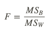
Recall that:

Between groups:

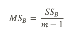
with m−1 degrees of freedom

Within groups:

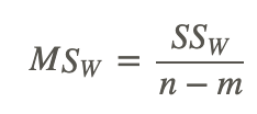
with n−m degrees of freedom

where:

n is the sample size of group k.

m is the total number of groups.

The degrees of freedom for the interaction is found by multiplying the degrees of freedom for the two variables.

Use these to fill out the table:

Source	Df	SS	MS	F
Smoking level	2	30850.4	15425.2	34.02
Gender	1	331.5	331.5	0.73
Interaction	2	4.58	2.29	0.005
Error	144	65297.52	453.455
Total	149	96484

Example 2

Conduct a significance test for a gender level effect. Clearly state your null and alternative hypotheses, your test statistic and your conclusion.

Null Hypothesis: In the population, the mean heart rate after six minutes is the same for males and females. Alternative Hypothesis: In the population, the mean heart rate after six minutes is different for males and females.

The value of the test statistic is F1,144=0.73. The p-value for this can be determined using the TI Calculator: Fcdf (.73, 10000000, 1, 144) = .394. Since this is larger than 0.05, we fail to reject the null hypothesis, which means that we conclude there is no difference in heart rate after 6 minutes across the levels of gender, male and female.

---

Review 

1. In two-way ANOVA, we study not only the effect of two independent variables on the dependent variable, but also the ___ between the two independent variables.
2. We could conduct multiple t-tests between pairs of hypotheses, but there are several advantages when we conduct a two-way ANOVA. These include:
   1. Efficiency
   2. Control over additional variables
   3. The study of interaction between variables
   4. All of the above
3. Calculating the total variation in two-way ANOVA includes calculating ___ types of variation.
   1. 1
   2. 2
   3. 3
   4. 4
4. A researcher is interested in determining the effects of different doses of a dietary supplement on the performance of both males and females on a physical endurance test. The three different doses of the medicine are low, medium, and high, and again, the genders are male and female. He assigns 48 people, 24 males and 24 females, to one of the three levels of the supplement dosage and gives a standardized physical endurance test. Using technological tools, he generates the following summary ANOVA table:

Source	SS	df	MS	F	Critical Value of F
Rows (gender)	14.832	1	14.832	14.94	4.07
Columns (dosage)	17.120	2	8.560	8.62	3.23
Interaction	2.588	2	1.294	1.30	3.23
Within-cell	41.685	42	992
Total	76,226	47

∗α=0.05

a. What are the three hypotheses associated with the two-way ANOVA method?

b. What are the three null hypotheses for this study?

c. What are the critical values for each of the three hypotheses? What do these tell us?

d. Would you reject the null hypotheses? Why or why not?

e. In your own words, describe what these results tell us about this experiment.

5. For each of the following two-way ANOVA situations specify the response variable, the two factors A and B, the number of categories in each factor and the number of levels for Factor A and B.
   1. One hundred overweight women are classified by whether they drink alcohol or not. They are randomly assigned to participate in a swimming program, a jogging program, or a yoga program. Weight loss after two months is measured.
   2. A random sample of first grade children in a certain state is given a reading test. The children are categorized by whether they attended preschool (not at all, some, regularly) and whether they have older siblings at home.
6. A commuter has a choice of three different routes (Factor A) to take to work and is interested in knowing if any of them are faster than the others. She suspects the day of the week might make a difference – Monday, middle of the week or Friday (Factor B). She takes ten observations on each of the possible combinations for a total of 90 measurements. Her response variable is commute time. Following is a table of mean times:

	Monday	Middle of week	Friday
Route 1	34.2	30.8	32.1
Route 2	22.7	24.6	26.0
Route 3	38.6	34.1	32.9

She has determined the following: SSA = 1868.9, SSB = 65, SSAB = 229.33, SSE = 552.8.

a. construct an ANOVA table for this data.

b. State the null and alternative hypotheses in the context of this problem for

i. A factor A effect

ii. A factor B effect

iii. An interaction between the factors

c. Conduct the hypothesis test for this situation for

i. A factor A effect

ii. A factor B effect

iii. An interaction between the factors.

7. Complete the following two-way ANOVA table:

Source	Df	SS	MS	F
Factor A	2	450
Factor B		840
Interaction	2	130
Error	48	1050
Total	53	2470

8. For the table in problem seven, carry out the hypothesis test for each of the following;
   1. Factor A
   2. Factor B
   3. Interaction AB
9. A researcher is investigating the general effects of smoking on physical activity capacity. She finds 9 nonsmokers, 9 moderate smokers and 9 heavy smokers as test subjects. She then assigns three people from each category to each of the physical activities.
   1. What type of test would you run on this data?
   2. What would the null hypotheses be?
10. Suppose you are the director of a tutoring agency and you want to determine if students who prepare for a particular standardized test with you agency do better on the standardized test. You obtain standardized test scores from students at three different universities who did and did not prepare through your agency. What is your model and what statistical test would you use to answer your question?

---

Review (Answers)

To view the Review answers, open this PDF file and look for section 11.3. 

---

Vocabulary

Term	Definition
the interaction effect	The interaction effect is the variation between the independent variables.
two way ANOVA	A two-way ANOVA allows you to study the effect of two independent variables and also the interaction between these variables.
variation within the group	Variation with the group is the cell-variation.
variations among the column means	Variations among column means is the variation in the dependent variable attributed to the other independent variable.
variations among the row means	Variations among row means is the variation in the dependent variable attributed to one independent variable.

---

Additional Resources

Video: One-Way ANOVA

Practice: ANOVA Tests