2.7.2: Tangent Graphs

Adjust the length of the curve, or the distance before the y values repeat, from $2\pi$.

Your mission, should you choose to accept it, as Agent Trigonometry is to find the period and the zeros of the function $y=\dfrac{1}{2}\tan 4x$.

Graph of a Tangent Function

The graph of the tangent function is very different from the sine and cosine functions. First, recall that the tangent ratio is $\tan \theta =\dfrac{\text{opposite}}{\text{adjacent}}$. In radians, the coordinate for the tangent function would be $(\theta ,\tan \theta )$

$\begin{array}{lllllllll}x & \theta & 0 & \dfrac{\pi}{6} & \dfrac{\pi}{4} & \dfrac{\pi}{3} \dfrac{\pi}{2} & \dfrac{2 \pi}{3} & \dfrac{3 \pi}{4} & \dfrac{3 \pi}{6} & \pi \\ y &\tan \theta &0 &\dfrac{\sqrt{3}}{3}&1 &\sqrt{3}\;\text{und. } &-\sqrt{3} &-1 &-\dfrac{\sqrt{3}}{3} &0 \end{array}$

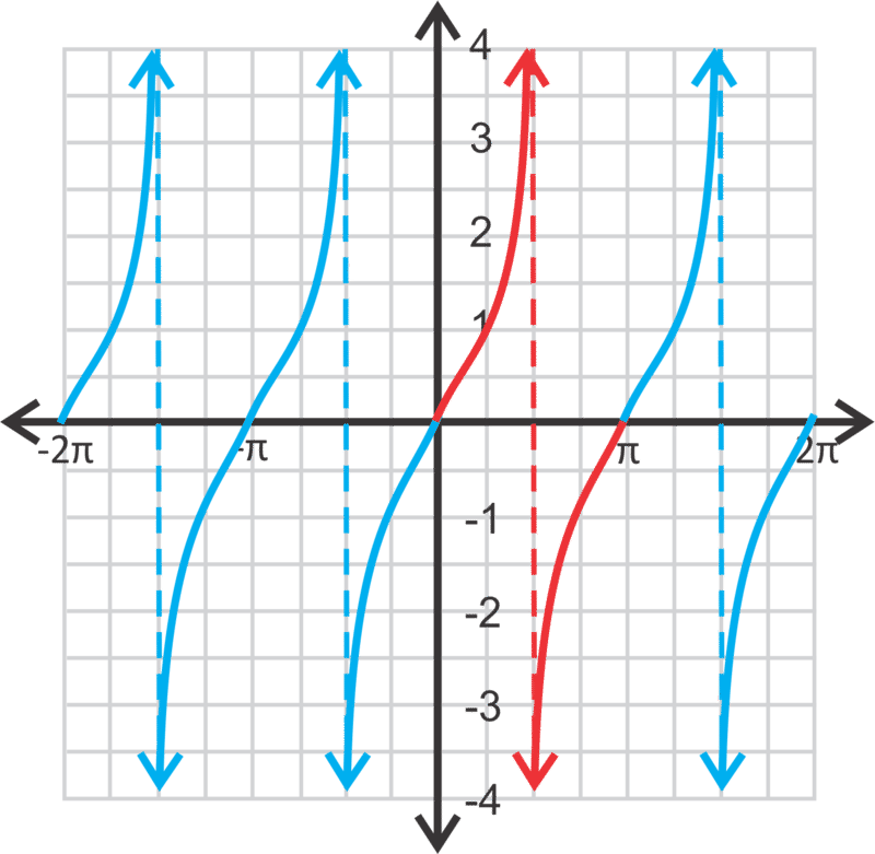
After $\pi$, the y-values repeat, making the tangent function periodic with a period of $\pi$.

Figure $\PageIndex{1}$

The red portion of the graph represents the coordinates in the table above. Repeating this portion, we get the entire tangent graph. Notice that there are vertical asymptotes at $x=−\dfrac{3\pi }{2}$, $−\dfrac{\pi }{2}$, $\dfrac{\pi }{2}$ and $\dfrac{3\pi }{2}$. If we were to extend the graph out in either direction, there would continue to be vertical asymptotes at the odd multiples of \pi 2. Therefore, the domain is all real numbers, $x\neq n\pi \pm \dfrac{\pi }{2}$, where $n$ is an integer. The range would be all real numbers. Just like with sine and cosine functions, you can change the amplitude, phase shift, and vertical shift.

The standard form of the equation is $y=a\tan b(x−h)+k$ where $a$, $b$, $h$, and $k$ are the same as they are for the other trigonometric functions. For simplicity, we will not address phase shifts (k) in this concept.

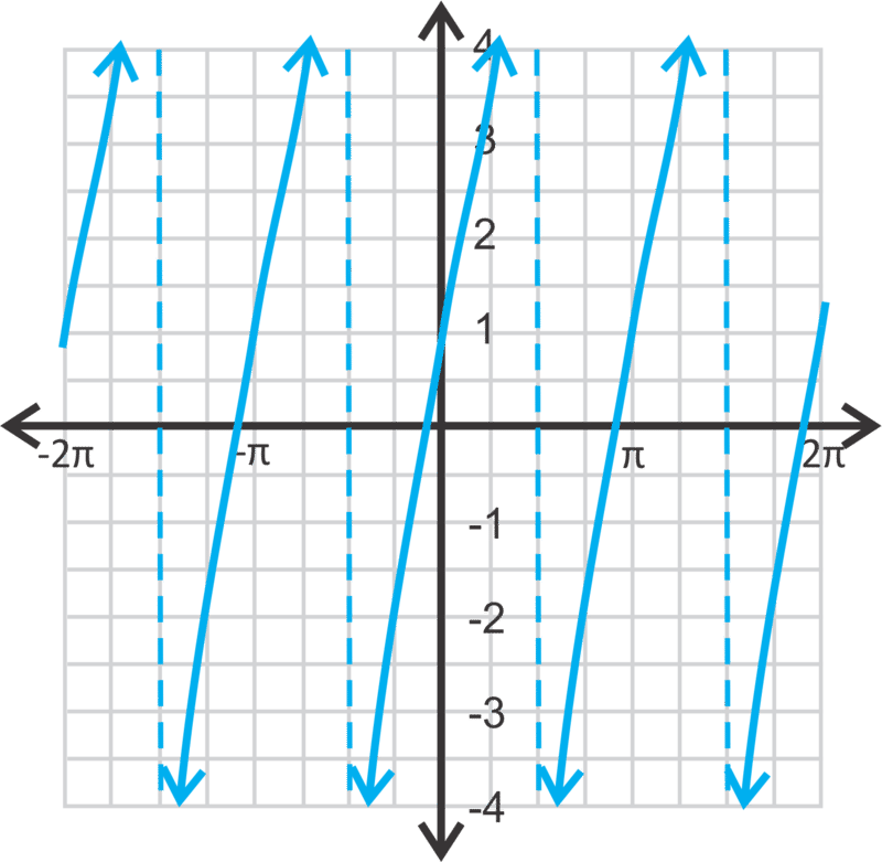
Let's graph $y=3\tan x+1$ from $[−2\pi ,2\pi ]$ and state the domain and range.

First, the amplitude is 3, which means each y-value will be tripled. Then, we will shift the function up one unit.

Figure $\PageIndex{2}$

Notice that the vertical asymptotes did not change. The period of this function is still $\pi$. Therefore, if we were to change the period of a tangent function, we would use a different formula than what we used for sine and cosine. To change the period of a tangent function, use the formula $\dfrac{\pi }{\mid b\mid }$.

The domain will be all real numbers, except where the asymptotes occur. Therefore, the domain of this function will be $x\in R$, $x\not\in n\pi \pm \dfrac{\pi }{2}$. The range is all real numbers.

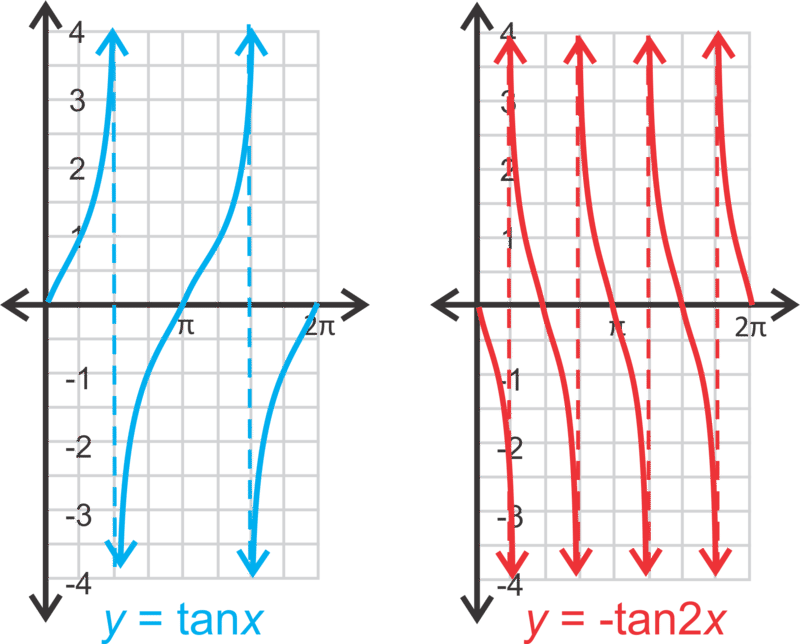
Now, let's graph $y=−\tan 2\pi$ from $[0,2\pi ]$, state the domain and range, and find all zeros within this domain.

The period of this tangent function will be $\dfrac{\pi }{2}$ and the curves will be reflected over the x-axis.

Figure $\PageIndex{3}$

The domain is all real numbers, $x\not\in \dfrac{\pi }{4}, \dfrac{3\pi }{4}, \dfrac{5\pi }{4}, \dfrac{7\pi }{4}, \dfrac{\pi }{4} \pm \dfrac{\pi }{2}n$ where $n$ is any integer. The range is all real numbers. To find the zeros, set $y=0$.

$\begin{aligned} 0 &=-\tan 2 x \\ 0 &=\tan 2 x \\ 2 x &=\tan ^{-1} 0=0, \pi, 2 \pi, 3 \pi, 4 \pi \\ x &=0, \dfrac{\pi}{2}, \pi, \dfrac{3 \pi}{2}, 2 \pi \end{aligned}$

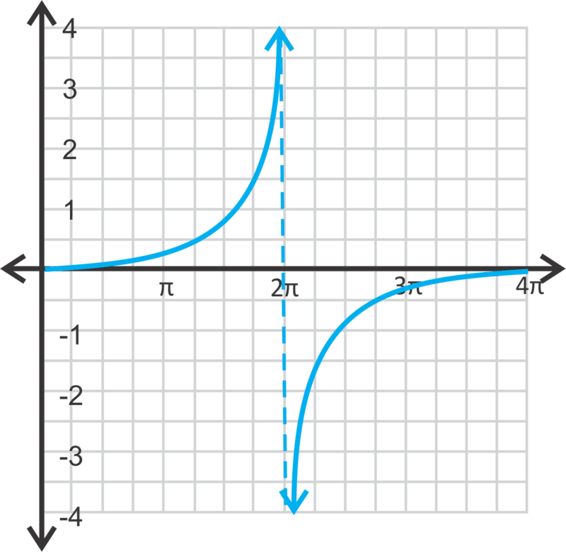
Finally, let's graph $y=\dfrac{1}{4}\tan \dfrac{1}{4}x$ from $[0,4\pi ]$ and state the domain and range.

This function has a period of $\dfrac{\pi }{\dfrac{1}{4}}=4\pi$. The domain is all real numbers, except $2\pi ,\; 6\pi ,\; 10\pi ,\; 2\pi \pm 4\pi n$, where $n$ is any integer. The range is all real numbers.

Figure $\PageIndex{4}$

Example $\PageIndex{1}$

Earlier, you were asked to find the period and zeros of the function $y=\dfrac{1}{2}\tan 4x$.

Solution

The period is $\dfrac{\pi }{4}$.

The zeros are where y is zero.

$\begin{aligned} 0&=\dfrac{1}{2} \tan 4 x \\ 0 &=\tan 4 x \\ 4 x &=\tan ^{-1} 0=0, \pi, 2 \pi, 3 \pi \\ x &=\dfrac{1}{4}(0, \pi, 2 \pi, 3 \pi) \\ x &=0, \dfrac{\pi}{4}, \dfrac{\pi}{2}, \dfrac{3}{4} \pi \end{aligned}$

Example $\PageIndex{2}$

Find the period of the function $y=−4\tan \dfrac{3}{2}x$.

Solution

The period is $\dfrac{\pi }{\dfrac{3}{2}}=\pi \cdot \dfrac{2}{3}=\dfrac{2\pi }{3}$.

Example $\PageIndex{3}$

Find the zeros of the function from Example 2, from $[0,2\pi ]$.

Solution

The zeros are where y is zero.

$\begin{aligned} 0 &=-4 \tan \dfrac{3}{2} x \\ 0 &=\tan \dfrac{3}{2} x \\ \dfrac{3}{2} x &=\tan ^{-1} 0=0, \pi, 2 \pi, 3 \pi \\ x &=\dfrac{2}{3}(0, \pi, 2 \pi, 3 \pi) \\ x &=0, \dfrac{2 \pi}{3}, \dfrac{4 \pi}{3}, 2 \pi \end{aligned}$

Example $\PageIndex{4}$

Find the equation of the tangent function with an amplitude of 8 and a period of $6\pi$.

Solution

The general equation is $y=a\tan bx$. We know that $a=8$. Let’s use the period to solve for the frequency, or $b$.

$\begin{aligned} \dfrac{\pi }{b}&=6\pi \\ b&=\dfrac{\pi }{6\pi }=\dfrac{1}{6}\end{aligned}$

The equation is $y=8\tan \dfrac{1}{6}x$.

Review

Graph the following tangent functions over $[0,4\pi ]$. Determine the period, domain, and range.

1. $y=2\tan x$
2. $y=−\dfrac{1}{3}\tan x$
3. $y=−\tan 3x$
4. $y=4\tan 2x$
5. $y=\dfrac{1}{2}\tan 4x$
6. $y=−\tan \dfrac{1}{2}x$
7. $y=4+\tan x$
8. $y=−3+\tan 3x$
9. $y=1+\dfrac{2}{3}\tan \dfrac{1}{2}x$
10. Find the zeros of the function from #1.
11. Find the zeros of the function from #3.
12. Find the zeros of the function from #5.

Write the equation of the tangent function, in the form $y=a\tan bx$, with the given amplitude and period.

13. Amplitude: 3 Period: $\dfrac{3\pi }{2}$
14. Amplitude: $\dfrac{1}{4}$ Period: $2\pi$
15. Amplitude: -2.5 Period: 8
16. Challenge Graph $y=2\tan \dfrac{1}{3}\left(x+\dfrac{\pi }{4}\right)−1$ over $[0,6\pi ]$. Determine the domain and period.

Answers for Review Problems

To see the Review answers, open this PDF file and look for section 14.5.

Additional Resource

Interactive Element