8.2: Confidence Intervals

Last updated
Save as PDF

Page ID: 5744

$ \newcommand{\vecs}[1]{\overset { \scriptstyle \rightharpoonup} {\mathbf{#1}} } $ $ \newcommand{\vecd}[1]{\overset{-\!-\!\rightharpoonup}{\vphantom{a}\smash {#1}}} $$\newcommand{\id}{\mathrm{id}}$ $ \newcommand{\Span}{\mathrm{span}}$ $ \newcommand{\kernel}{\mathrm{null}\,}$ $ \newcommand{\range}{\mathrm{range}\,}$ $ \newcommand{\RealPart}{\mathrm{Re}}$ $ \newcommand{\ImaginaryPart}{\mathrm{Im}}$ $ \newcommand{\Argument}{\mathrm{Arg}}$ $ \newcommand{\norm}[1]{\| #1 \|}$ $ \newcommand{\inner}[2]{\langle #1, #2 \rangle}$ $ \newcommand{\Span}{\mathrm{span}}$ $\newcommand{\id}{\mathrm{id}}$ $ \newcommand{\Span}{\mathrm{span}}$ $ \newcommand{\kernel}{\mathrm{null}\,}$ $ \newcommand{\range}{\mathrm{range}\,}$ $ \newcommand{\RealPart}{\mathrm{Re}}$ $ \newcommand{\ImaginaryPart}{\mathrm{Im}}$ $ \newcommand{\Argument}{\mathrm{Arg}}$ $ \newcommand{\norm}[1]{\| #1 \|}$ $ \newcommand{\inner}[2]{\langle #1, #2 \rangle}$ $ \newcommand{\Span}{\mathrm{span}}$$\newcommand{\AA}{\unicode[.8,0]{x212B}}$

Confidence Intervals

Sampling distributions are the connecting link between the collection of data by unbiased random sampling and the process of drawing conclusions from the collected data. Results obtained from a survey can be reported as a point estimate. For example, a single sample mean is a point estimate, because this single number is used as a plausible value of the population mean. Keep in mind that some error is associated with this estimate-the true population mean may be larger or smaller than the sample mean. An alternative to reporting a point estimate is identifying a range of possible values the parameter might take, controlling the probability that the parameter is not lower than the lowest value in this range and not higher than the largest value. This range of possible values is known as a confidence interval. Associated with each confidence interval is a confidence level. This level indicates the level of assurance you have that the resulting confidence interval encloses the unknown population mean.

In a normal distribution, we know that 95% of the data will fall within two standard deviations of the mean. Another way of stating this is to say that we are confident that in 95% of samples taken, the sample statistics are within plus or minus two standard errors of the population parameter. As the confidence interval for a given statistic increases in length, the confidence level increases.

The selection of a confidence level for an interval determines the probability that the confidence interval produced will contain the true parameter value. Common choices for the confidence level are 90%, 95%, and 99%. These levels correspond to percentages of the area under the normal density curve. For example, a 95% confidence interval covers 95% of the normal curve, so the probability of observing a value outside of this area is less than 5%. Because the normal curve is symmetric, half of the 5% is in the left tail of the curve, and the other half is in the right tail of the curve. This means that 2.5% is in each tail.

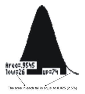
Screen Shot 2020-07-13 at 4.17.36 PM.png

The graph shown above was made using a TI-83 graphing calculator and shows a normal distribution curve for a set of data for which μ=50 and σ=12. A 95% confidence interval for the standard normal distribution, then, is the interval (−1.96, 1.96), since 95% of the area under the curve falls within this interval. The ±1.96 are the z-scores that enclose the given area under the curve. For a normal distribution, the margin of error is the amount that is added to and subtracted from the mean to construct the confidence interval. For a 95% confidence interval, the margin of error is 1.96σ. (Note that previously we said that 95% of the data in a normal distribution falls within ±2 standard deviations of the mean. This was just an estimate, and for the remainder of this textbook, we'll assume that 95% of the data actually falls within ±1.96 standard deviations of the mean.)

The following is the derivation of the confidence interval for the population mean, μ. In it, zα2 refers to the positive z-score for a particular confidence interval. The Central Limit Theorem tells us that the distribution of x¯ is normal, with a mean of μ and a standard deviation of σn‾√. Consider the following:

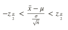
Screen Shot 2020-07-13 at 4.18.14 PM.png

All values are known except for μ. Solving for this parameter, we have:

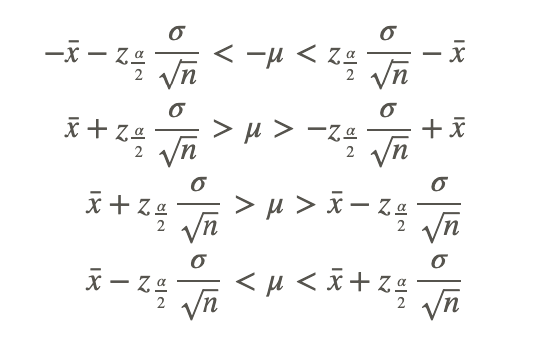
Screen Shot 2020-07-13 at 4.18.41 PM.png

Another way to express this is: 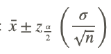Screen Shot 2020-07-13 at 4.19.06 PM.png

Calculations Involving Confidence Intervals

Jenny randomly selected 60 muffins of a particular brand and had those muffins analyzed for the number of grams of fat that they each contained. Rather than reporting the sample mean (point estimate), she reported the confidence interval. Jenny reported that the number of grams of fat in each muffin is between 10.3 grams and 12.1 grams with 95% confidence.

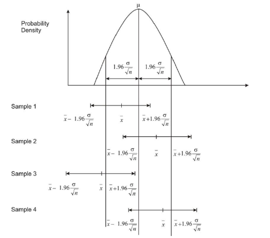
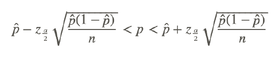
In this example, the population mean is unknown. This number is fixed, not variable, and the sample means are variable, because the samples are random. If this is the case, does the confidence interval enclose this unknown true mean? Random samples lead to the formation of confidence intervals, some of which contain the fixed population mean and some of which do not. The most common mistake made by persons interpreting a confidence interval is claiming that once the interval has been constructed, there is a 95% probability that the population mean is found within the confidence interval. Even though the population mean is unknown, once the confidence interval is constructed, either the mean is within the confidence interval, or it is not. Hence, any probability statement about this particular confidence interval is inappropriate. In the above example, the confidence interval is from 10.3 to 12.1, and Jenny is using a 95% confidence level. The appropriate statement should refer to the method used to produce the confidence interval. Jenny should have stated that the method that produced the interval from 10.3 to 12.1 has a 0.95 probability of enclosing the population mean. This means if she did this procedure 100 times, 95 of the intervals produced would contain the population mean. The probability is attributed to the method, not to any particular confidence interval. The following diagram demonstrates how the confidence interval provides a range of plausible values for the population mean and that this interval may or may not capture the true population mean. If you formed 100 intervals in this manner, 95 of them would contain the population mean.

Screen Shot 2020-07-13 at 4.20.22 PM.png

Interpreting Confidence Intervals

The following questions are to be answered with reference to the above diagram.

1. Were all four sample means within ^1.96σ/_n^.5, or ^1.96σ/_x̄, of the population mean? Explain.

The sample mean, x̄, for Sample 3 was not within ^1.96σ/_n^.5 of the population mean. It did not fall within the vertical lines to the left and right of the population mean.

2. Did all four confidence intervals capture the population mean? Explain.

The confidence interval for Sample 3 did not enclose the population mean. This interval was just to the left of the population mean, which is denoted with the vertical line found in the middle of the sampling distribution of the sample means.

3. In general, what percentage of x̄′s should be within ^1.96σ/_n^0.5 of the population mean?

95%

4. In general, what percentage of the confidence intervals should contain the population mean?

95%

When the sample size is large (n>30), the confidence interval for the population mean is calculated as shown below:

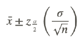Screen Shot 2020-07-13 at 4.22.45 PM.png , where z_^α/2 is 1.96 for a 95% confidence interval, 1.645 for a 90% confidence interval, and 2.58 for a 99% confidence interval.

Determining Confidence Intervals

Julianne collects four samples of size 60 from a known population with a population standard deviation of 19 and a population mean of 110. Using the four samples, she calculates the four sample means to be:

107 112 109 115

1. For each sample, determine the 90% confidence interval.

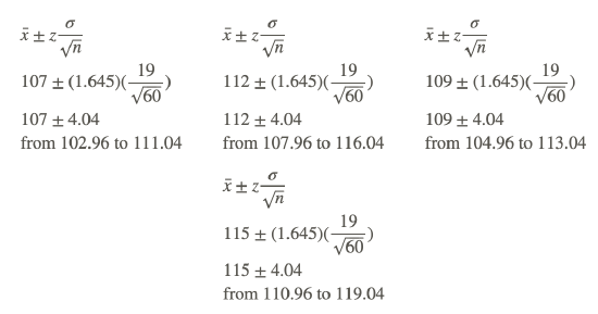
Screen Shot 2020-07-13 at 4.23.38 PM.png

2. Do all four confidence intervals enclose the population mean? Explain.

Three of the confidence intervals enclose the population mean. The interval from 110.96 to 119.04 does not enclose the population mean.

Confidence Intervals for Hypotheses about Population Proportions

Often statisticians are interested in making inferences about a population proportion. For example, when we look at election results we often look at the proportion of people that vote and who this proportion of voters choose. Typically, we call these proportions percentages and we would say something like “Approximately 68 percent of the population voted in this election and 48 percent of these voters voted for Barack Obama.”

In estimating a parameter, we can use a point estimate or an interval estimate. The point estimate for the population proportion, p, is p̂. We can also find interval estimates for this parameter. These intervals are based on the sampling distributions of p̂.

If we are interested in finding an interval estimate for the population proportion, the following two conditions must be satisfied:

We must have a random sample.
The sample size must be large enough (np̂ >10 and n(1−p̂ )>10) that we can use the normal distribution as an approximation to the binomial distribution.

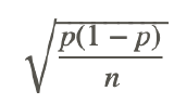Screen Shot 2020-07-13 at 4.27.15 PM.png is the standard deviation of the distribution of sample proportions. The distribution of sample proportions is as follows:

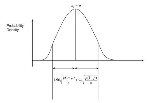
Screen Shot 2020-07-13 at 4.26.44 PM.png

Since we do not know the value of p, we must replace it with p̂ . We then have the standard error of the sample proportions,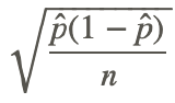 Screen Shot 2020-07-13 at 4.29.35 PM.png . If we are interested in a 95% confidence interval, using the Empirical Rule, we are saying that we want the difference between the sample proportion and the population proportion to be within 1.96 standard deviations.

That is, we want the following:

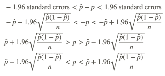
Screen Shot 2020-07-13 at 4.30.05 PM.png

This is a 95% confidence interval for the population proportion. If we generalize for any confidence level, the confidence interval is as follows:

Screen Shot 2020-07-15 at 4.03.16 PM.png

In other words, the confidence interval is 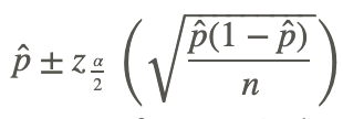Screen Shot 2020-07-15 at 4.03.58 PM.png .

Remember that z_^α/2 refers to the positive z-score for a particular confidence interval. Also, p̂ is the sample proportion, and n is the sample size. As before, the margin of error is 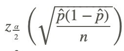Screen Shot 2020-07-15 at 4.05.06 PM.png , and the confidence interval is p̂ ± the margin of error.

Calculating Confidence Intervals for Proportions

A congressman is trying to decide whether to vote for a bill that would remove all speed limits on interstate highways. He will decide to vote for the bill only if 70 percent of his constituents favor the bill. In a survey of 300 randomly selected voters, 224 (74.6%) indicated they would favor the bill. The congressman decides that he wants an estimate of the proportion of voters in the population who are likely to favor the bill. Construct a confidence interval for this population proportion.

Our sample proportion is 0.746, and our standard error of the proportion is 0.0251. We will construct a 95% confidence interval for the population proportion. Under the normal curve, 95% of the area is between z=−1.96 and z=1.96. Thus, the confidence interval for this proportion would be:

0.746±(1.96)(0.0251)

0.697<p<0.795

With respect to the population proportion, we are 95% confident that the interval from 0.697 to 0.795 contains the population proportion. The population proportion is either in this interval, or it is not. When we say that this is a 95% confidence interval, we mean that if we took 100 samples, all of size n, and constructed 95% confidence intervals for each of these samples, 95 out of the 100 confidence intervals we constructed would capture the population proportion, p.

Technology Note: Simulation of Random Samples and Formation of Confidence Intervals on the TI-83/84 Calculator

Now it is time to use a graphing calculator to simulate the collection of three samples of sizes 30, 60, and 90, respectively. The three sample means will be calculated, as well as the three 95% confidence intervals. The samples will be collected from a population that displays a normal distribution, with a population standard deviation of 108 and a population mean of 2130. We will use the randNorm( function found in [MATH], under the PRB menu. First, store the three samples in L1, L2, and L3, respectively, as shown below:

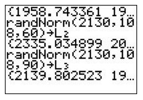
Screen Shot 2020-07-15 at 4.05.55 PM.png

Store 'randNorm(μ,σ,n)' in L1. The sample size is n=30.

Store 'randNorm(μ,σ,n)' in L2. The sample size is n=60.

Store 'randNorm(μ,σ,n)' in L3. The sample size is n=90.

The lists of numbers can be viewed by pressing [STAT][ENTER]. The next step is to calculate the mean of each of these samples.

To do this, first press [2ND][LIST] and go to the MATH menu. Next, select the 'mean(' command and press [2ND][L1][ENTER]. Repeat this process for L2 and L3.

Note that your confidence intervals will be different than the ones calculated below, because the random numbers generated by your calculator will be different, and thus, your means will be different. For us, the means of L1, L2, and L3 were 2139.1, 2119.2, and 2137.1, respectively, so the confidence intervals are as follows:

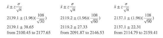
Screen Shot 2020-07-15 at 4.06.34 PM.png

As was expected, the value of x̄ varied from one sample to the next. The other fact that was evident was that as the sample size increased, the length of the confidence interval became smaller, or decreased. This is because with the increase in sample size, you have more information, and thus, your estimate is more accurate, which leads to a narrower confidence interval.

In all of the examples shown above, you calculated the confidence intervals for the population mean using the formula 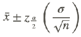Screen Shot 2020-07-15 at 4.07.20 PM.png . However, to use this formula, the population standard deviation σ had to be known. If this value is unknown, and if the sample size is large (n>30), the population standard deviation can be replaced with the sample standard deviation. Thus, the formula 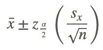can be used as an interval estimator, or confidence interval. This formula is valid only for simple random samples. Since 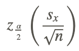Screen Shot 2020-07-15 at 4.08.40 PM.png is the margin of error, a confidence interval can be thought of simply as: x̄± the margin of error.

Using Technology

A committee set up to field-test questions from a provincial exam randomly selected grade 12 students to answer the test questions. The answers were graded, and the sample mean and sample standard deviation were calculated. Based on the results, the committee predicted that on the same exam, 9 times out of 10, grade 12 students would have an average score of within 3% of 65%.

1. Are you dealing with a 90%, 95%, or 99% confidence level?

You are dealing with a 90% confidence level. This is indicated by 9 times out of 10.

2. What is the margin of error?

The margin of error is 3%.

3. Calculate the confidence interval.

The confidence interval is the mean plus or minus the margin of error, or 62% to 68%

4. Explain the meaning of the confidence interval.

There is a 0.90 probability that the method used to produce this interval from 62% to 68% results in a confidence interval that encloses the population mean (the true score for this provincial exam).

Examples

A large grocery store has been recording data regarding the number of shoppers that use savings coupons at its outlet. Last year, it was reported that 77% of all shoppers used coupons, and 19 times out of 20, these results were considered to be accurate within 2.9%.

Example 1

Are you dealing with a 90%, 95%, or 99% confidence level?

The statement 19 times out of 20 indicates that you are dealing with a 95% confidence interval.

Example 2

What is the margin of error?

The results were accurate within 2.9%, so the margin of error is 0.029.

Example 3

Calculate the confidence interval.

The confidence interval is simply p̂ ± the margin of error.

77%−2.9%=74.1%
77%+2.9%=79.9%

Thus, the confidence interval is from 0.741 to 0.799.

Example 4

Explain the meaning of the confidence interval.

The 95% confidence interval from 0.741 to 0.799 for the population proportion is an interval calculated from a sample by a method that has a 0.95 probability of capturing the population proportion.

Review

In a local teaching district, a technology grant is available to teachers in order to install a cluster of four computers in their classrooms. From the 6,250 teachers in the district, 250 were randomly selected and asked if they felt that computers were an essential teaching tool for their classroom. Of those selected, 142 teachers felt that computers were an essential teaching tool.
1. Calculate a 99% confidence interval for the proportion of teachers who felt that computers are an essential teaching tool.
2. How could the survey be changed to narrow the confidence interval but to maintain the 99% confidence interval?
Josie followed the guidelines presented to her and conducted a binomial experiment. She did 300 trials and reported a sample proportion of 0.61.
1. Calculate the 90%, 95%, and 99% confidence intervals for this sample.
2. What did you notice about the confidence intervals as the confidence level increased? Offer an explanation for your findings?
3. If the population proportion were 0.58, would all three confidence intervals enclose it? Explain.
Does replacing σ with s change your chance of capturing the unknown population mean? Is there a way to increase the chance of capturing the unknown population mean?

A study was conducted to determine the mean birth weight of a certain breed of kittens. Consider the birth weights of kittens to be normally distributed. A sample of 45 kittens was randomly selected from all kittens of this breed at a large veterinary hospital. The birth weight of each kitten in the sample was recorded. The sample mean was 3.56 ounces, and the sample standard deviation was 0.2 ounces. Set a 90% confidence interval on the mean birth weight of all kittens of this breed.
In a study of seventh grade students, the mean number of hours per week that they watched television was 18.7 with a standard deviation of 4.5 hours. Assume the population has a normal distribution. Construct a 95% confidence interval for the mean number of hours of tv watched by seventh grade students.
A random sample of 40 college students has mean annual earnings of $3,245 and a standard deviation of $567. Construct a 99% confidence interval for the population. Does the population have to follow a normal distribution? Explain.
A random sample of 16 light bulbs has a mean life of 650 hours and a standard deviation of 32 hours. Assume the population has a normal distribution. Construct a 90% confidence interval for the population mean.
A sample of 100 cans of peas showed an average weight of 14 ounces with a standard deviation of 0.7 ounces. Construct a 95% confidence interval for the mean of the population.
What three factors affect the width of a confidence interval for a population mean? For each factor, indicate how an increase in the numerical value of the factor affects the interval width.
For each of the following use the information given to calculate the standard error of the mean and find an approximate 90% confidence interval for the population mean:
1. n=81,x̄=64.2,s=2.7
2. n=100,x̄=123.5,s=9
3. n=324,x̄=123.5,s=9
Suppose a random sample of 64 men has a mean foot length of 27.5 cm with a standard deviation of 2 cm.
1. Calculate the standard error of the sample mean.
2. Calculate an approximate 99% confidence interval for the mean foot length of men. Write a sentence that interprets this interval.
For each combination of sample size and sample proportion find the approximate margin of error for the 90% confidence interval:
1. n=100,p̂ =0.56
2. n=400,p̂ =0.56
3. n=400,p̂ =0.25
4. n=400,p̂ =0.75
Suppose a new cancer treatment is given to a sample of 300 patients. The treatment was successful for 210 of the patients. Assume that these patients are representative of the population of individuals who have this cancer.
1. Calculate the sample proportion that was successfully treated.
2. Determine a 90% confidence interval for the proportion successful treated. Write a sentence that interprets this interval.
Suppose a polling organization reports that the margin of error is 3% for a sample survey. Explain what this indicates about the possible difference between a percent determined from the survey data and the population value of the percent.
A poll conducted in the United States November 8 – 15, 2010 asked “The Secretary of Transportation recently said that he may push Congress for a national ban on using a cell phone while driving. The ban would include hands-free cell phones. Do you think that a national ban on using a cell phone while driving is a good idea or a bad idea?" In the nationwide poll of n=2,424 registered voters 63% said they thought it was a good idea. The margin of error was reported as ±2%. (source: wwwlpollingreport.com).
1. Find a 95% confidence interval estimate of the percent of American voters who believe banning cell phones when driving is a good idea at the time of the poll.
2. Write a sentence that interprets the interval computed in part (a).
A Gallup Organization telephone poll of 511 adults, aged 18 and older, living in the continental United States found that 70% of Americans feel confident in the accuracy of their doctor's advice, and don't feel the need to check for a second opinion or do additional research. The margin of error for this survey was given as ±5percentage points.
1. Find a 95% confidence interval estimate of the percent of American adults who feel confident in the accuracy of their doctor’s advice and don’t feel the need to check for a second opinion.
2. Based on the interval you found, is it reasonable to say that more than 65% of American voting adults have confidence in their doctor’s advice?
Suppose 100 researchers each plan to independently gather data and construct 95% confidence interval for a population mean. If X= the number of those intervals that actually cover the population mean, then Xis a binomial random variable.
1. What is a “success” for this random variable?
2. What is the numerical value of the probability of success?
3. What is the expected number of intervals that will cover their population means?
In computing the confidence interval for a population mean, μ, explain whether the interval would be wider, more narrow, or neither as a result of each of the following changes:
1. The level of confidence is changed from 85% to 90%.
2. The sample size is tripled.
3. A new random sample of the same size is taken and is increased by 10.
Calculate a 98% confidence interval for the proportion successfully treated in problem 13. Is this interval wider or narrower than the interval computed in problem 12?
In a Gallup Youth Survey done in 2000, 501 randomly selected American teenagers were asked about how well they get along with their parents.
1. According to the Gallup Organization, the margin of error for the poll was 5%. Verify that this figure is approximately correct.
2. A survey result was that 54% of the sample said they get along “very well” with their parents. Using the reported margin of error, calculate a 90% confidence interval for the population proportion that gets along “very well” with their parents.
3. Using the more exact margin of error, calculate a 90% confidence interval. Compare your answer to part (b).
Determine the value of the z∗ multiplier that would be used to compute an 80% confidence interval for a population proportion.

Review (Answers)

To view the Review answers, open this PDF file and look for section 7.3.

Vocabulary

Term	Definition
confidence intervals	A confidence interval is the interval within which you expect to capture a specific value. The confidence interval width is dependent on the confidence level.
confidence level	A confidence level is the probability value associated with a confidence interval.
margin of error	The margin of error is found by multiplying the standard error of the mean by the z-score of the percent confidence level
point estimate	A point estimate of a population parameter is a single value used to estimate the population parameter.
population proportion	For qualitative variables, the population proportion is a parameter of interest.

Additional Resources

Video: What are Confidence Intervals?

Practice: Confidence Intervals

Real World: Close Calls